Clustering features - IgG Standardized - AP vs WP only
Excluding total IgG - 6 response clusters
Lisa Gallagher, David Kook, Scot Zens
2024-09-11
Last updated: 2024-09-11
Checks: 6 1
Knit directory:
madi-project3-sdy8003-pertussis-thailand/
This reproducible R Markdown analysis was created with workflowr (version 1.7.1). The Checks tab describes the reproducibility checks that were applied when the results were created. The Past versions tab lists the development history.
The R Markdown is untracked by Git. To know which version of the R
Markdown file created these results, you’ll want to first commit it to
the Git repo. If you’re still working on the analysis, you can ignore
this warning. When you’re finished, you can run
wflow_publish to commit the R Markdown file and build the
HTML.
Great job! The global environment was empty. Objects defined in the global environment can affect the analysis in your R Markdown file in unknown ways. For reproduciblity it’s best to always run the code in an empty environment.
The command set.seed(20231106) was run prior to running
the code in the R Markdown file. Setting a seed ensures that any results
that rely on randomness, e.g. subsampling or permutations, are
reproducible.
Great job! Recording the operating system, R version, and package versions is critical for reproducibility.
Nice! There were no cached chunks for this analysis, so you can be confident that you successfully produced the results during this run.
Great job! Using relative paths to the files within your workflowr project makes it easier to run your code on other machines.
Great! You are using Git for version control. Tracking code development and connecting the code version to the results is critical for reproducibility.
The results in this page were generated with repository version 6485bfa. See the Past versions tab to see a history of the changes made to the R Markdown and HTML files.
Note that you need to be careful to ensure that all relevant files for
the analysis have been committed to Git prior to generating the results
(you can use wflow_publish or
wflow_git_commit). workflowr only checks the R Markdown
file, but you know if there are other scripts or data files that it
depends on. Below is the status of the Git repository when the results
were generated:
Ignored files:
    Ignored:    .RData
    Ignored:    .Renviron
    Ignored:    .Rhistory
    Ignored:    .Rproj.user/
    Ignored:    8clusters-vaccinated-APvs.WP-IgGStandardized.pdf
    Ignored:    NULL
    Ignored:    code/cluster_functions_lisa.R
    Ignored:    output/

Untracked files:
    Untracked:  analysis/boxplot_arm_apwp.Rmd
    Untracked:  analysis/cluster_features_nosigg_apwp_noELISA6_tangle_DKAB.Rmd
    Untracked:  analysis/cluster_features_sigg_apwp_noELISA6_tangle_DKAB.Rmd
    Untracked:  analysis/cluster_features_sigg_apwp_noIgG6_tangle_DKAB.Rmd
    Untracked:  analysis/cluster_features_sigg_apwp_noIgG7_tangle_DKAB.Rmd
    Untracked:  code/clusters_features_nosigg_apwp_noEL7_DK.RData
    Untracked:  code/clusters_features_nosigg_matpm_noEL7_DK.RData
    Untracked:  code/clusters_features_sigg_matpm_noEL7_DK.RData
    Untracked:  code/clusters_features_stand_igg_apwp_noEL7_DK.RData
    Untracked:  code/clusters_features_stand_igg_apwp_noIgG7_DK.RData
    Untracked:  code/clustersbyarm_features_nosigg_apwp_noEL7_DK.RData
    Untracked:  code/clustersbyarm_features_nosigg_apwp_noIgG7_DK.RData
    Untracked:  code/clustersbyarm_features_nosigg_matpm_noEL7_DK.RData
    Untracked:  code/clustersbyarm_features_nosigg_matpm_noIgG7_DK.RData
    Untracked:  code/clustersbyarm_features_sigg_apwp_noEL7_DK.RData
    Untracked:  code/clustersbyarm_features_sigg_apwp_noIgG7_DK.RData
    Untracked:  code/clustersbyarm_features_sigg_matpm_noEL7_DK.RData
    Untracked:  code/clustersbyarm_features_sigg_matpm_noIgG7_DK.RData
    Untracked:  code/tanglegram_function_alec.R
    Untracked:  code/tdata_rxna_stand_igg_apwp_noEL7.RData

Unstaged changes:
    Modified:   analysis/cluster_features_nosigg_apwp_noELISA7_tangle_DKAB.Rmd
    Modified:   analysis/cluster_features_sigg_apwp_noELISA7_tangle_DKAB.Rmd
    Modified:   analysis/feature_estimates_matpm.Rmd
    Modified:   analysis/index_apwp.Rmd
    Modified:   code/cluster_functions.R
    Modified:   code/colors.R
Note that any generated files, e.g. HTML, png, CSS, etc., are not included in this status report because it is ok for generated content to have uncommitted changes.
There are no past versions. Publish this analysis with
wflow_publish() to start tracking its development.
Overview: AP vs. WP - Clustering features at the month 7 (vaccinated) and month 19 (boosted) visits
Data are log transformed and scaled AFTER removing the variance related to Total IgG for each feature separately by visit.
Missing data are excluded from this analysis.
Hierarchical clustering is based on a similarity matrix based on absolute rank correlation: 1 - abs(cor(num_tdata_scaled))
By Visit - vaccinated : Results
Heatmap clustering
Cluster Arms

[1] “after_cluster_arms”
Fix Arms
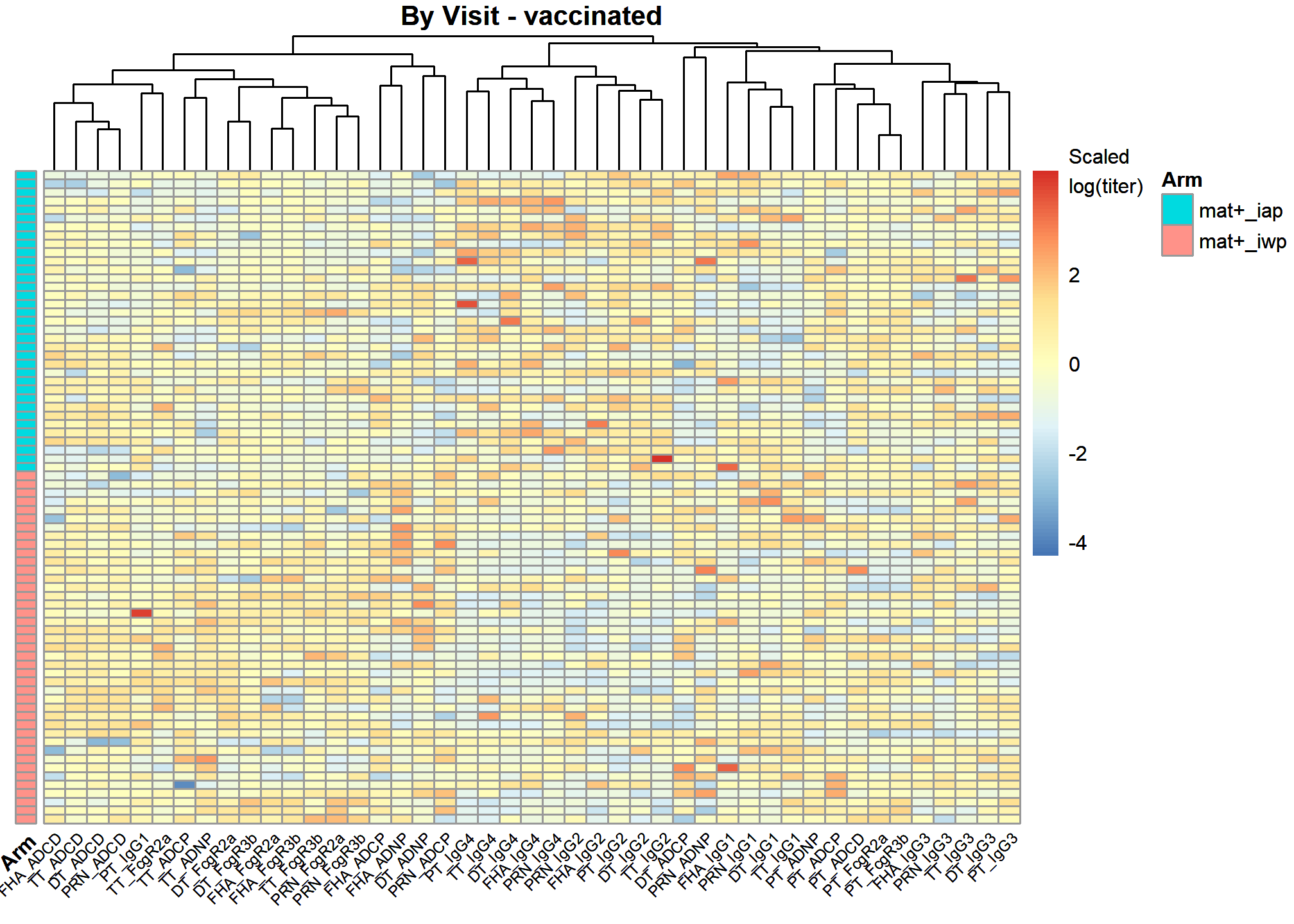
[1] “after_fix_arms”
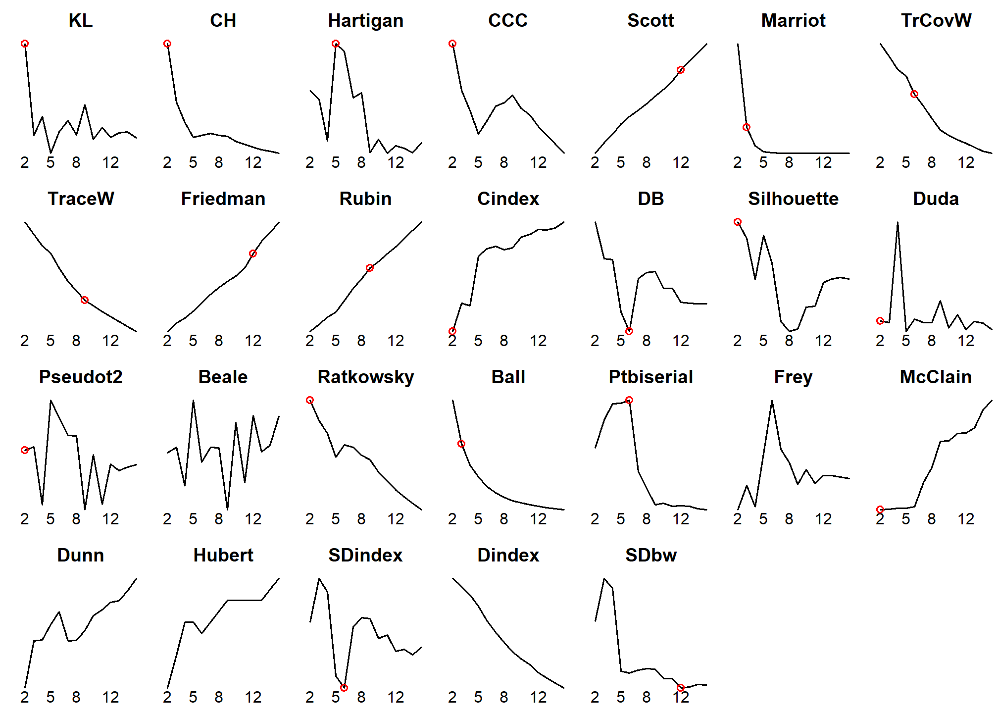
Number of Clusters
Among all indices:
9 proposed 2 as the best number of clusters
2 proposed 3 as the best number of clusters
1 proposed 5 as the best number of clusters
4 proposed 6 as the best number of clusters
2 proposed 9 as the best number of clusters
3 proposed 12 as the best number of clusters
2 proposed 15 as the best number of clusters
***** Conclusion *****According to the majority rule, the best number of clusters is 2
Dendrogram
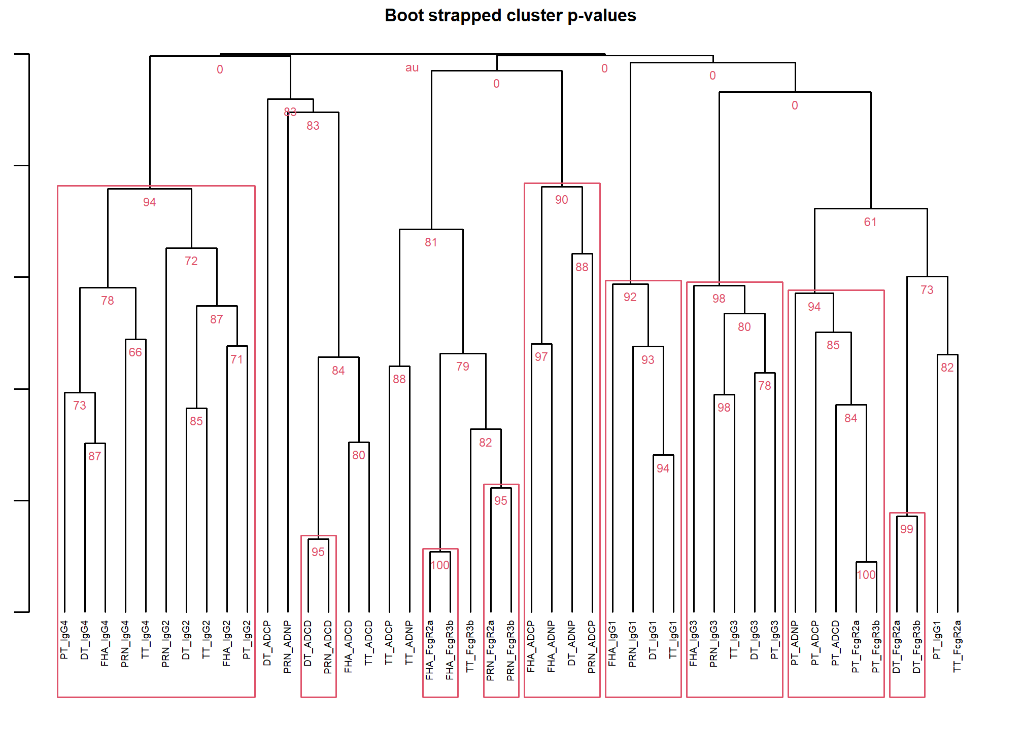
Whole feature set clustering: basic clusters and tree branch boot strap tests
[1] “after_dendrogram”
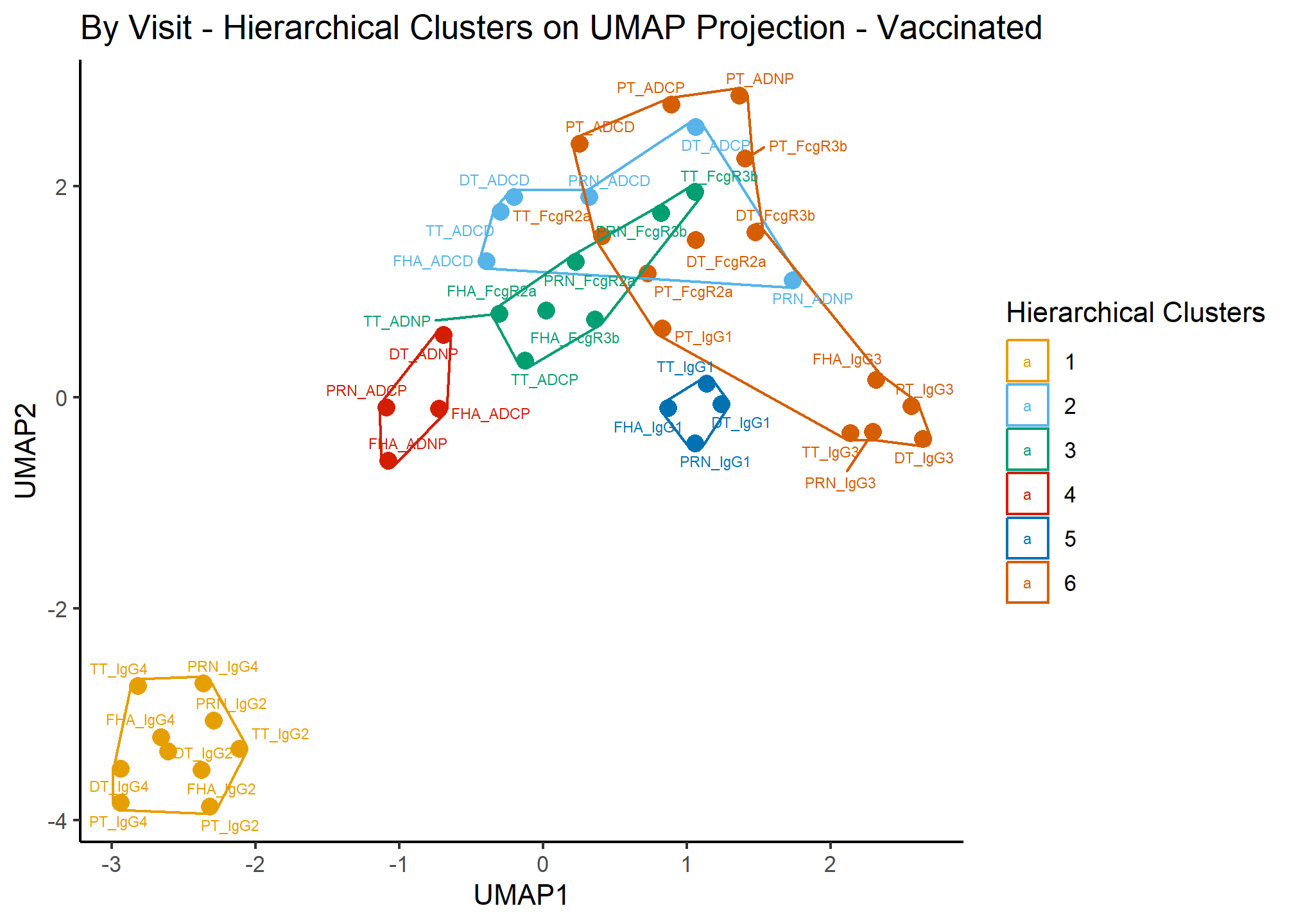
Hierarchical Clusters
The number of clusters shown is optimized using the preponderance of indicies for this purpose.
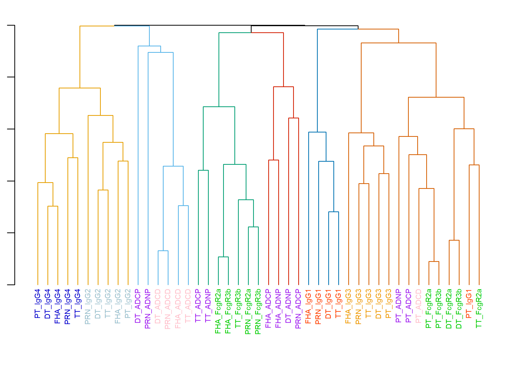
[1] “after_dendlistnew”
Tree Branch Tests
References
Suzuki, R. and Shimodaira, H. (2006) Pvclust: an R package for assessing the uncertainty in hierarchical clustering, Bioinformatics, 22 (12): 1540-1542.
Shimodaira, H. (2004) Approximately unbiased tests of regions using multistep-multiscale bootstrap resampling, Annals of Statistics, 32, 2616-2641.
Shimodaira, H. (2002) An approximately unbiased test of phylogenetic tree selection, Systematic Biology, 51, 492-508.
Suzuki, R. and Shimodaira, H. (2004) An application of multiscale bootstrap resampling to hierarchical clustering of microarray data: How accurate are these clusters?, The Fifteenth International Conference on Genome Informatics 2004, P034.
UMAP Concordance
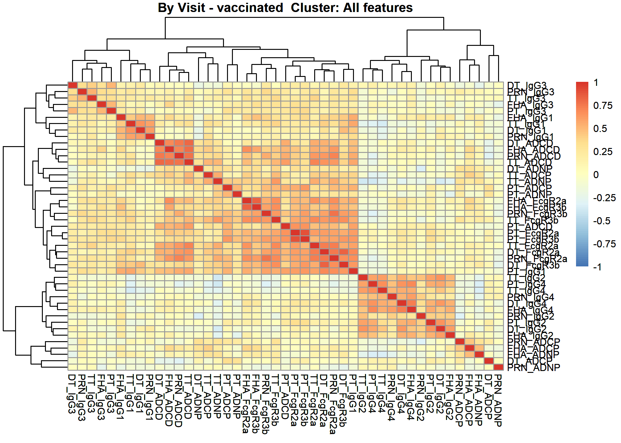
Correlation Heatmap: all features
These heatmaps are based on Spearman Rank Correlation.
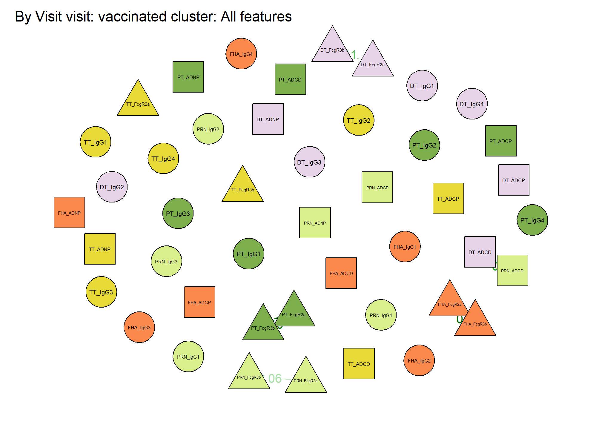
Correlation Network: all features
The correlation networks are based on Partial Correlation. This means that all the correlation between pairs of features after all the other correlation is accounted for. Sometimes there are sparse networks when no significant partial correlation left to plot. Sometimes there are too few samples for the number of features and the correlation matrix becomes indefinite. In either of these circumstances no network plot will be made.
 From
To Weight 4 — 5 0.11 13 — 14 0.17 1 — 19 0.15 22 — 23 0.06 31 — 32
0.19
From
To Weight 4 — 5 0.11 13 — 14 0.17 1 — 19 0.15 22 — 23 0.06 31 — 32
0.19
Cluster Contents
| name | contents |
|---|---|
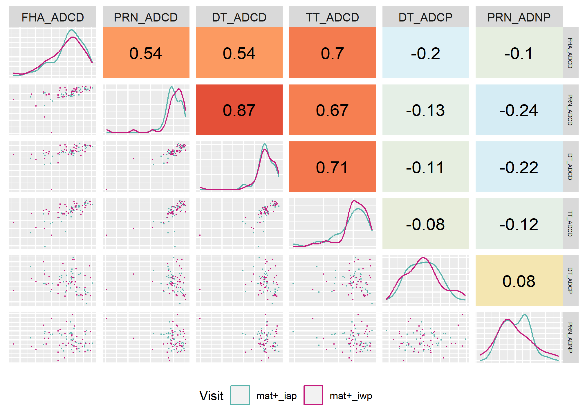
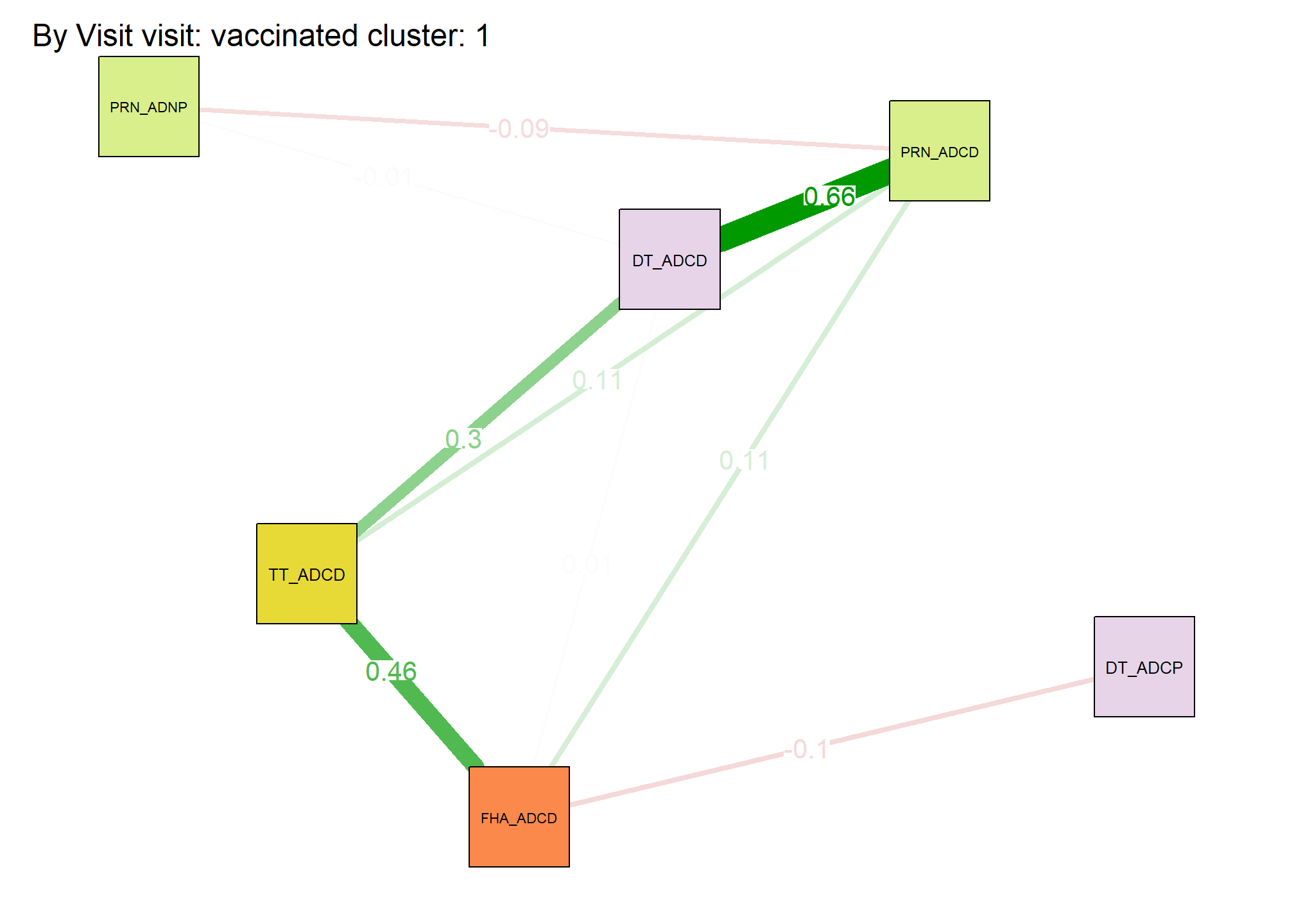
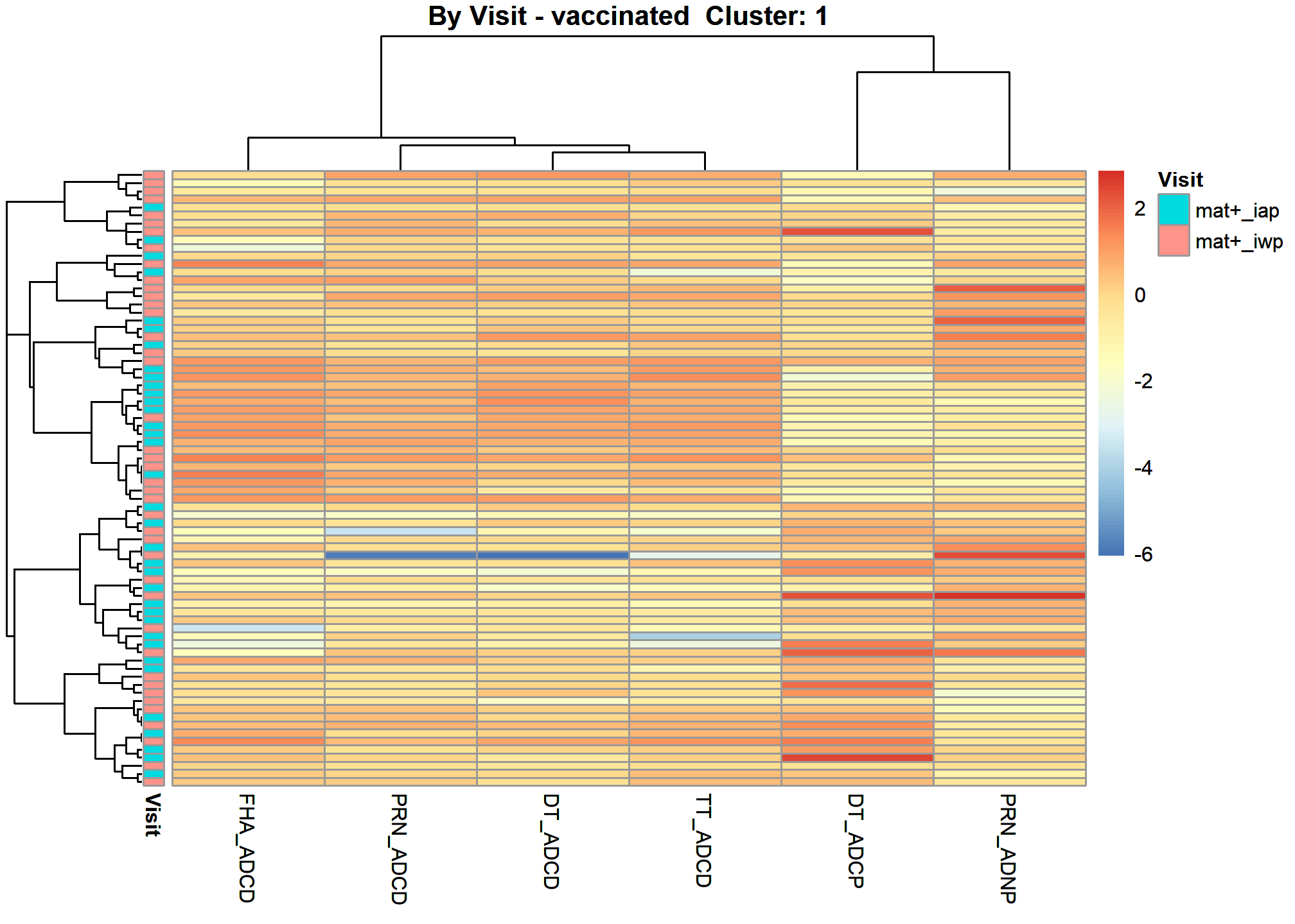
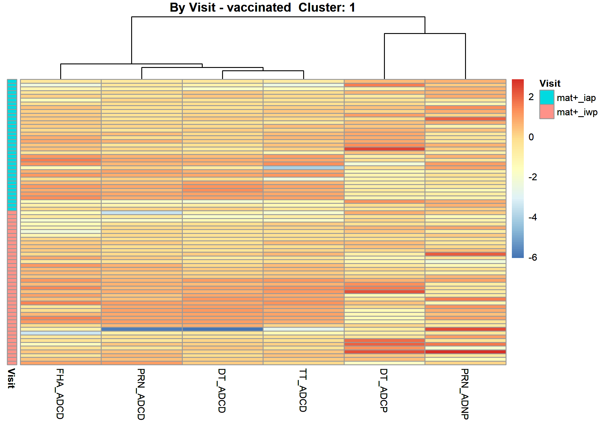
| Cluster_1 | DT_ADCD, DT_ADCP, FHA_ADCD, PRN_ADCD, PRN_ADNP, TT_ADCD |
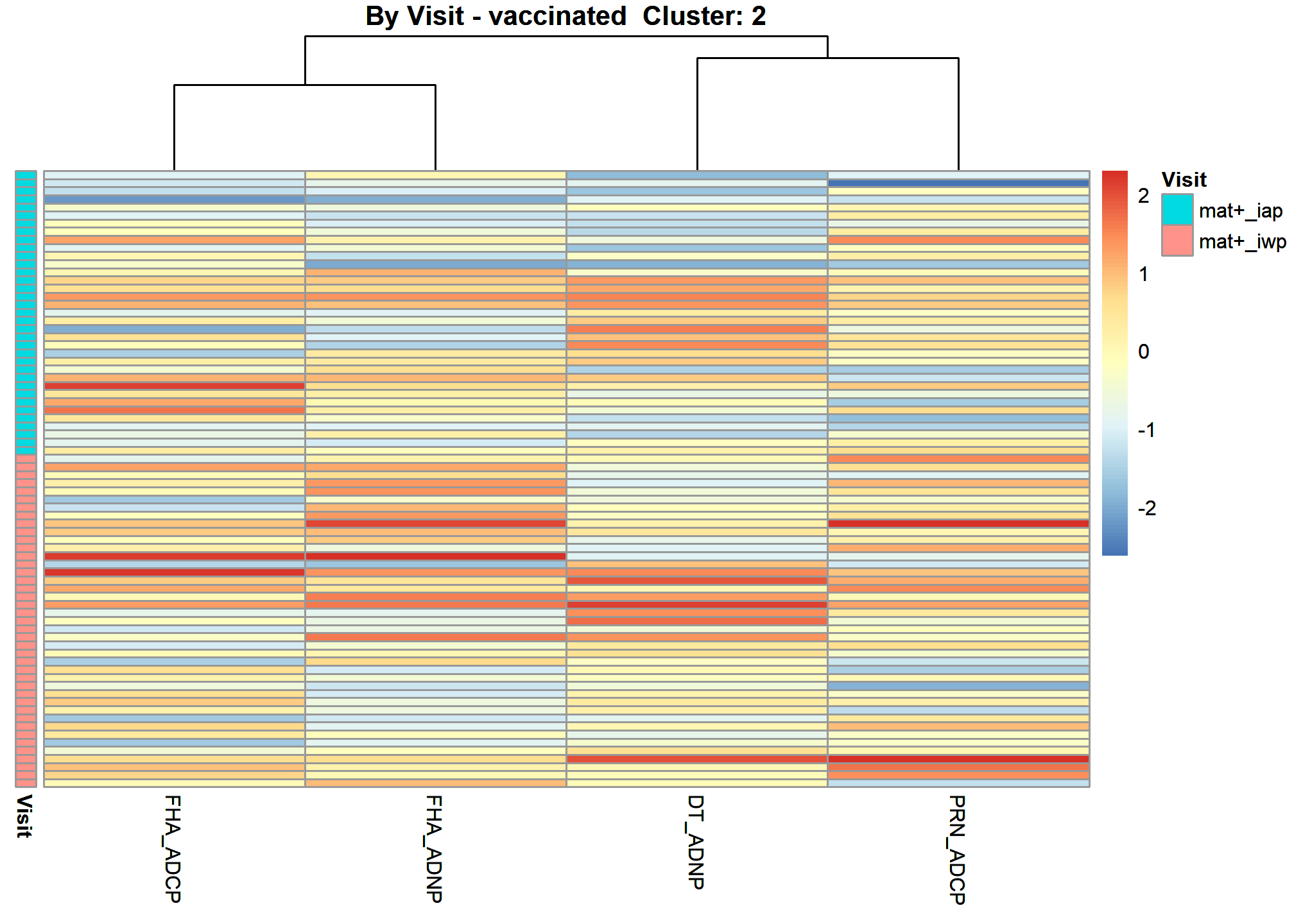
| Cluster_2 | DT_ADNP, FHA_ADCP, FHA_ADNP, PRN_ADCP |
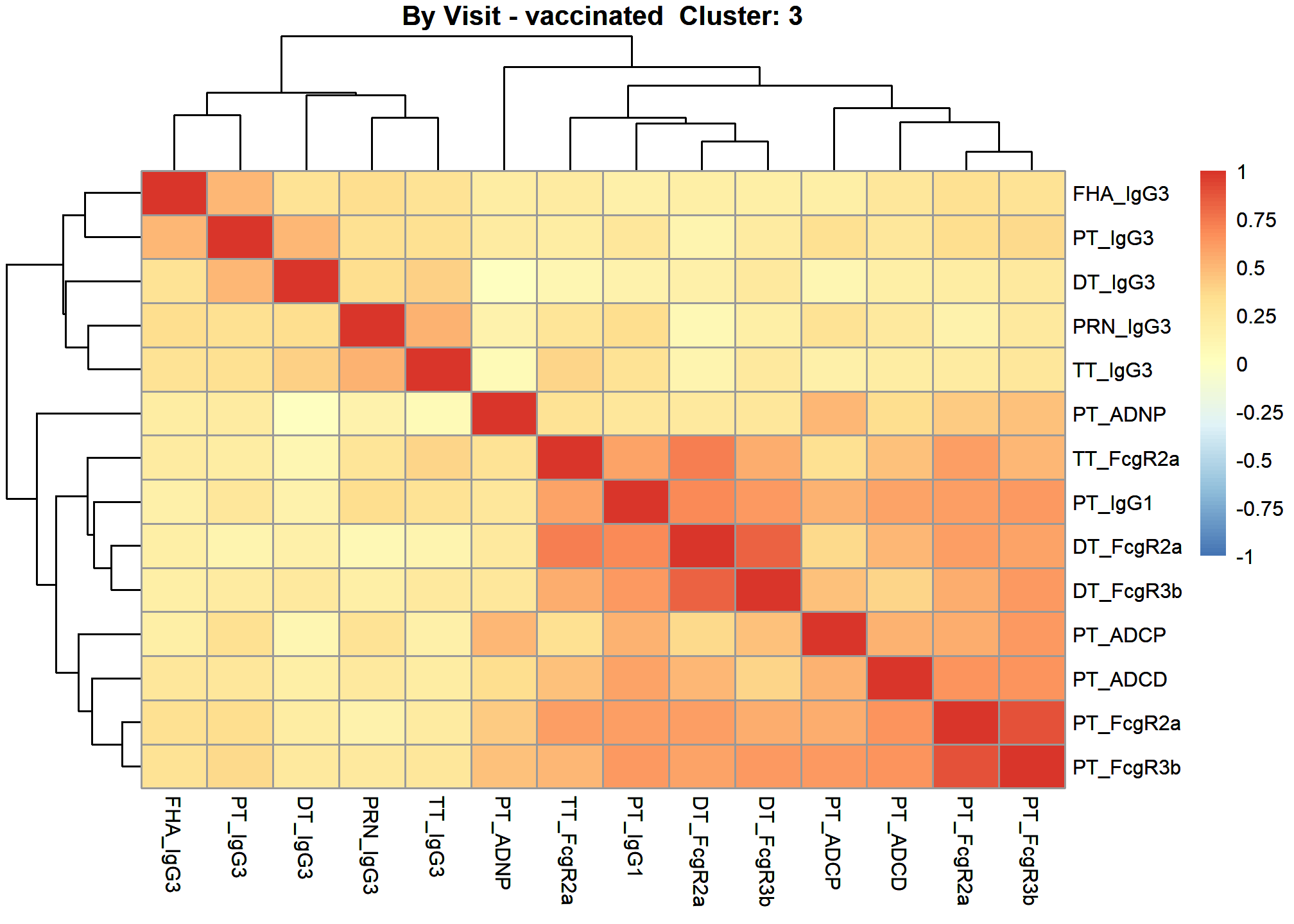
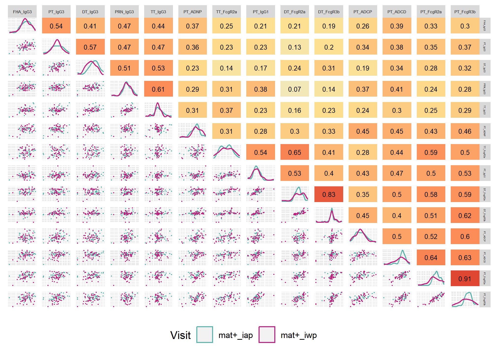
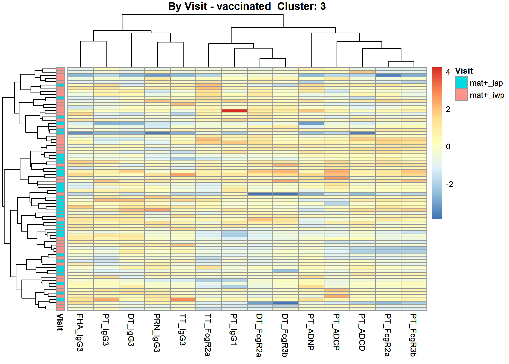
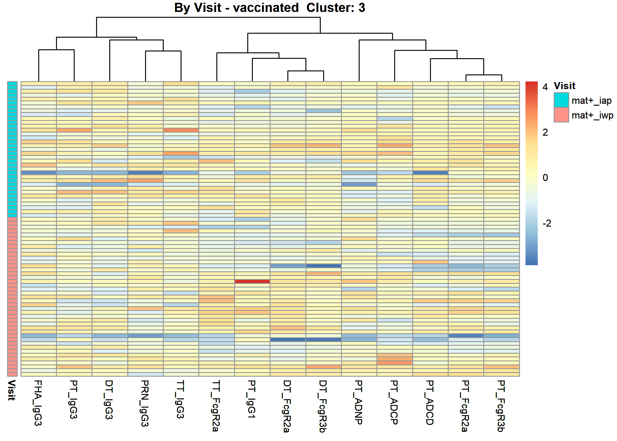
| Cluster_3 | DT_FcgR2a, DT_FcgR3b, DT_IgG3, FHA_IgG3, PRN_IgG3, PT_ADCD, PT_ADCP, PT_ADNP, PT_FcgR2a, PT_FcgR3b, PT_IgG1, PT_IgG3, TT_FcgR2a, TT_IgG3 |
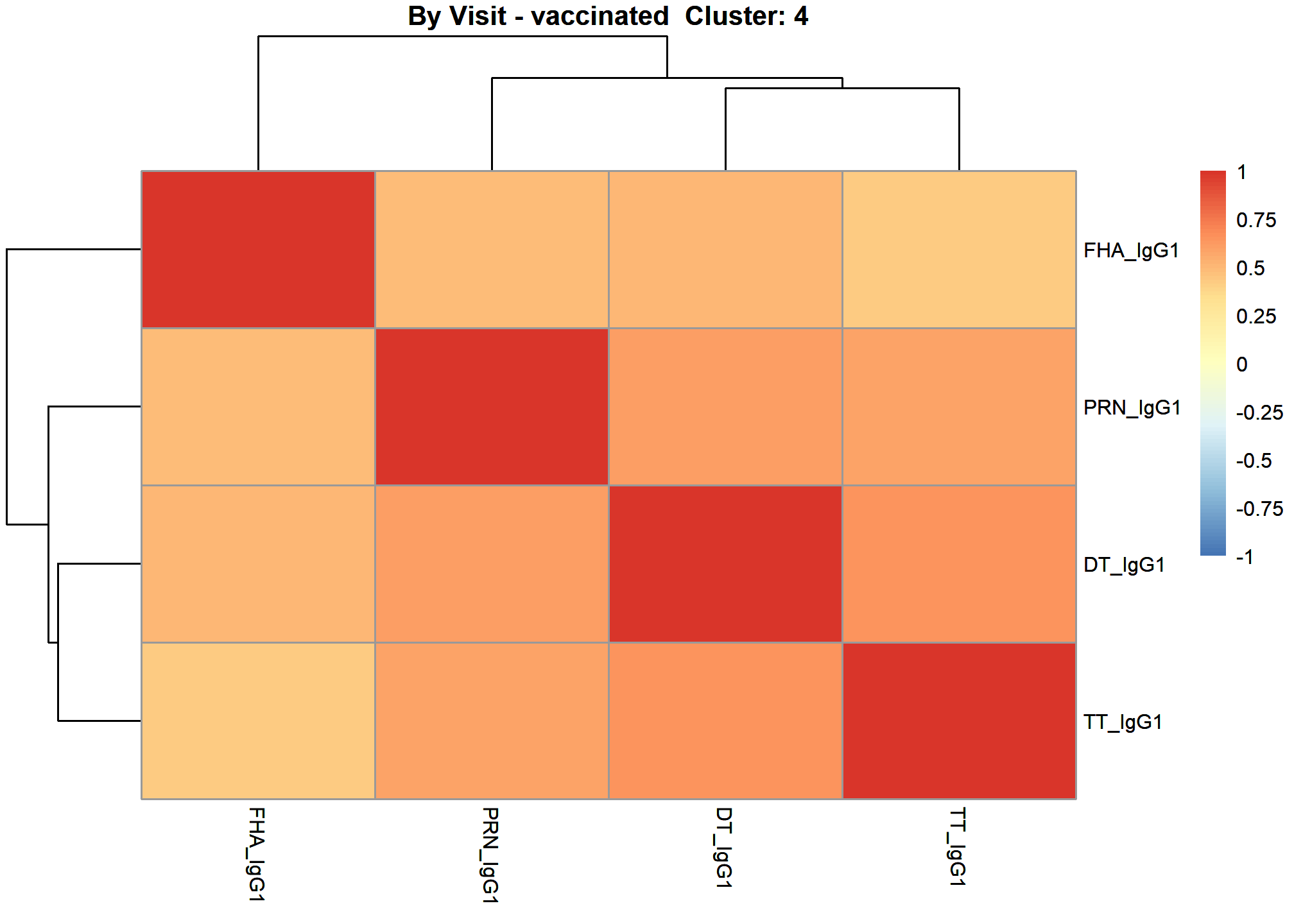
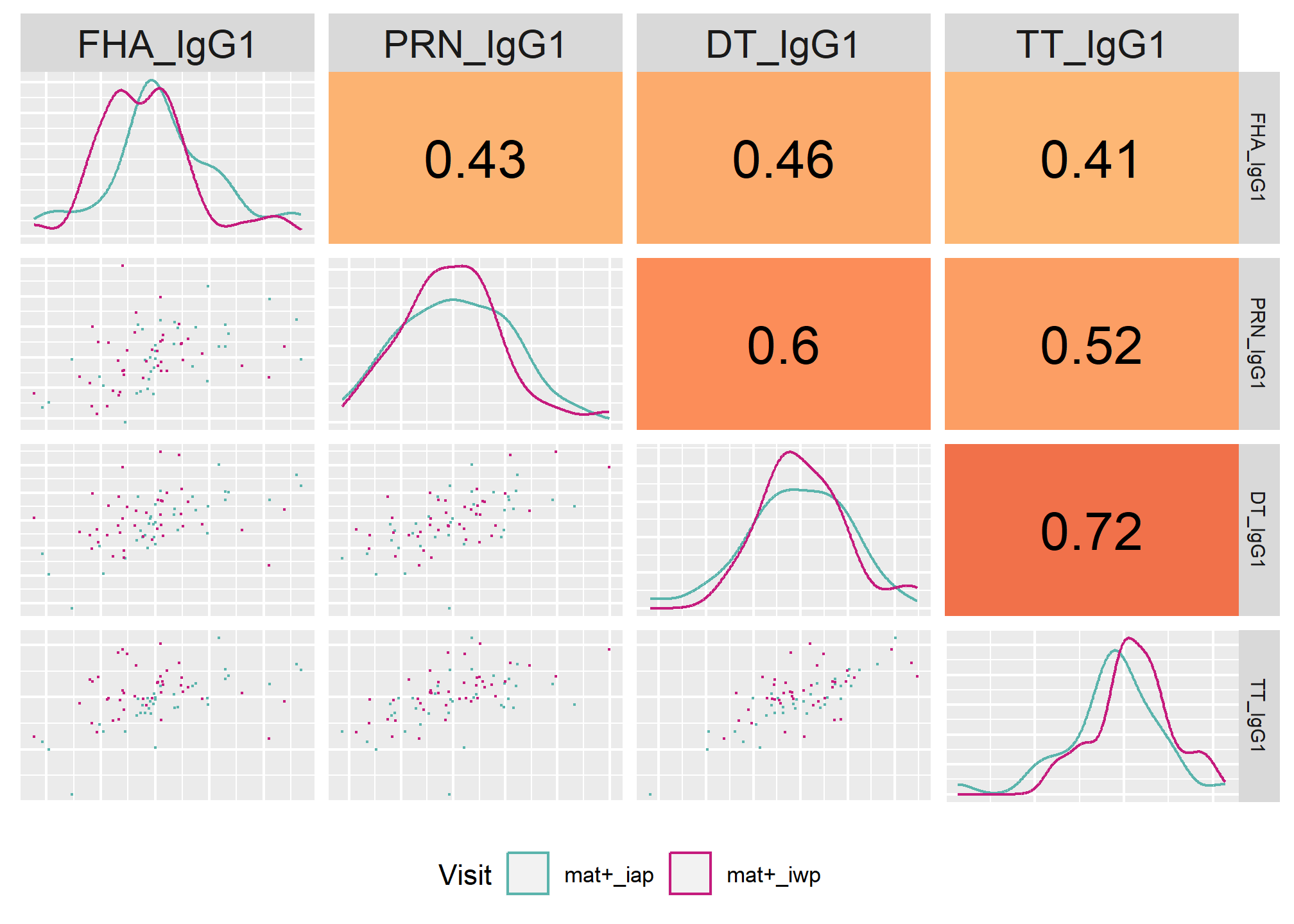
| Cluster_4 | DT_IgG1, FHA_IgG1, PRN_IgG1, TT_IgG1 |
| Cluster_5 | DT_IgG2, DT_IgG4, FHA_IgG2, FHA_IgG4, PRN_IgG2, PRN_IgG4, PT_IgG2, PT_IgG4, TT_IgG2, TT_IgG4 |
| Cluster_6 | FHA_FcgR2a, FHA_FcgR3b, PRN_FcgR2a, PRN_FcgR3b, TT_ADCP, TT_ADNP, TT_FcgR3b |
Cluster 1
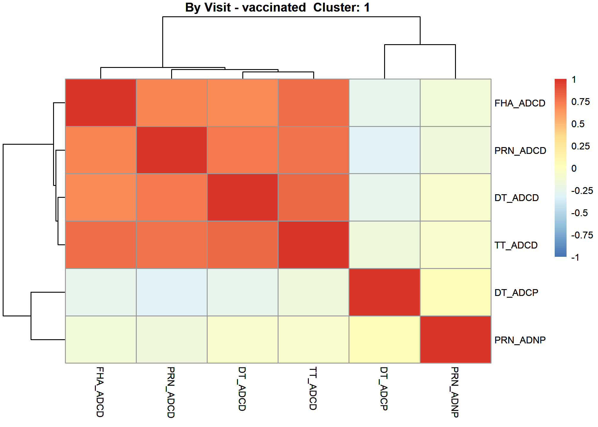
[1] “DT_ADCD” “DT_ADCP” “FHA_ADCD” “PRN_ADCD” “PRN_ADNP” “TT_ADCD”
Correlation Heatmap 1
These heatmaps are based on Spearman Rank Correlation.
 [1]
“after cluster specific correlation heatmap”
[1]
“after cluster specific correlation heatmap”
 [1]
“after cluster specific correlation scatter plot grid”
[1]
“after cluster specific correlation scatter plot grid”
Correlation Network 1
The correlation networks are based on optimal sparse estimates of the partial correlation matrix (Friedman, Hastie and Tibshirani, 2011). Partial correlations represent the remaining association (-1,1) between two nodes after controlling for all other node associations (Epskamp, S. & Fried, Eiko I. (2018)). The lines between nodes are labelled with the partial correlation coefficient. Sometimes there are sparse networks when no significant partial correlation left to plot. Sometimes there are too few samples for the number of features and the correlation matrix becomes indefinite. In either of these circumstances no network plot will be made.
 From
To Weight 1 — 3 0.01 2 — 3 -0.1 1 — 4 0.66 3 — 4 0.11 1 — 5 -0.01 4 — 5
-0.09 1 — 6 0.3 3 — 6 0.46 4 — 6 0.11
From
To Weight 1 — 3 0.01 2 — 3 -0.1 1 — 4 0.66 3 — 4 0.11 1 — 5 -0.01 4 — 5
-0.09 1 — 6 0.3 3 — 6 0.46 4 — 6 0.11
Heatmap Subjects Clustered 1
Heatmap Arm Assigned 1
Cluster 2
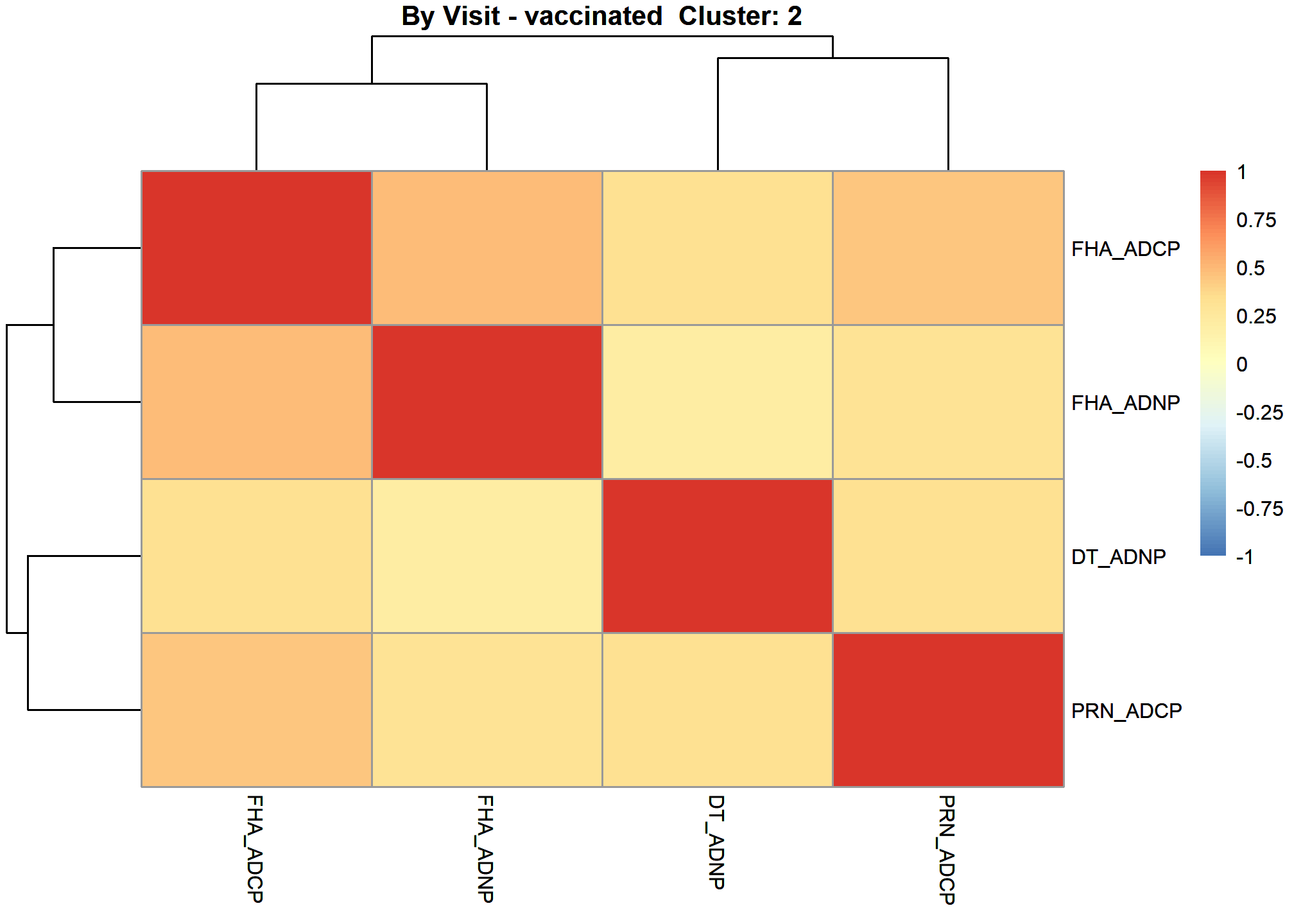
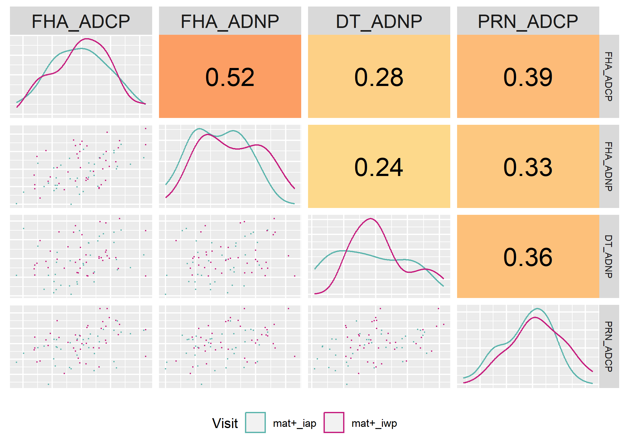
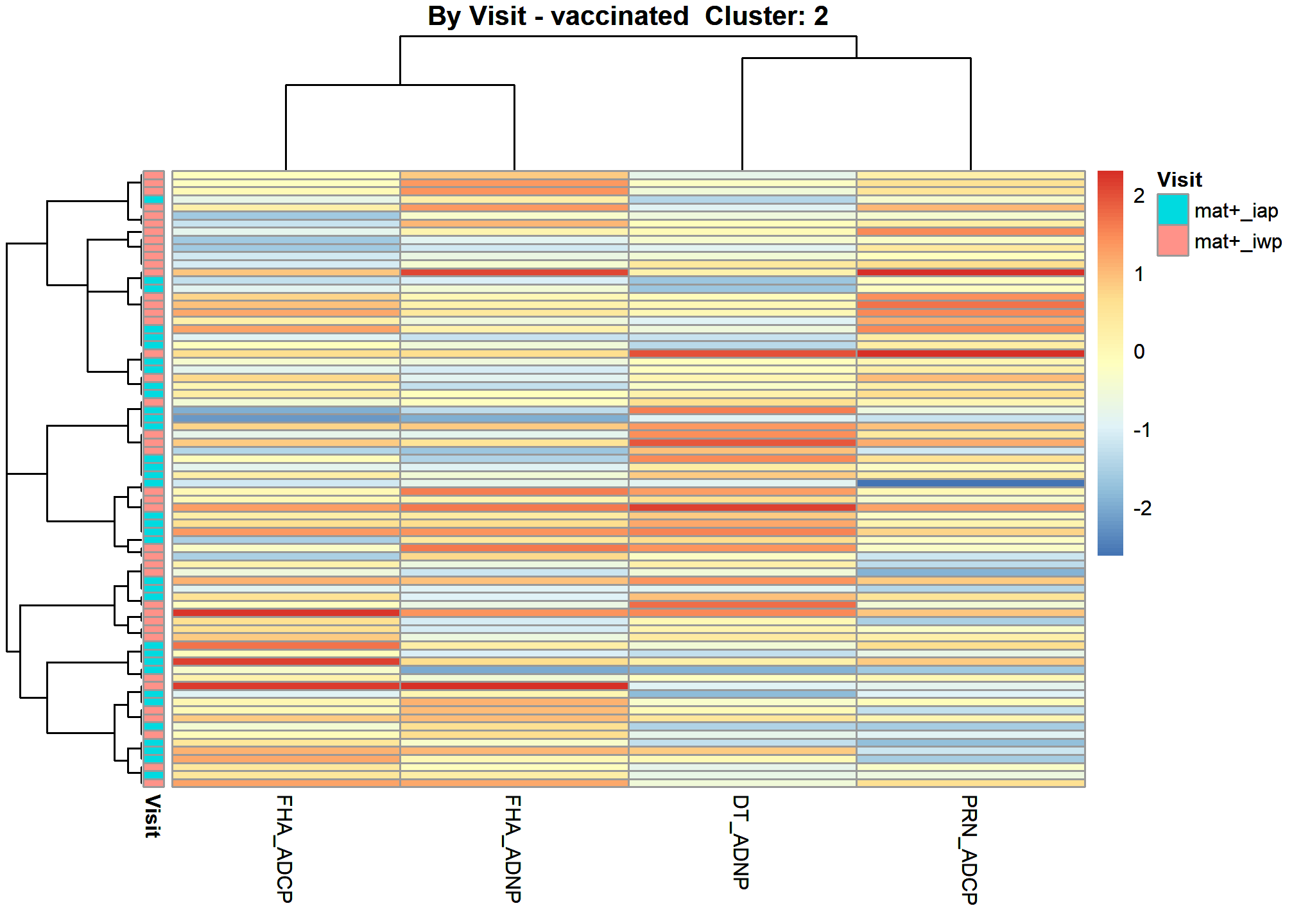
[1] “DT_ADNP” “FHA_ADCP” “FHA_ADNP” “PRN_ADCP”
Correlation Heatmap 2
These heatmaps are based on Spearman Rank Correlation.
 [1]
“after cluster specific correlation heatmap”
[1]
“after cluster specific correlation heatmap”
 [1]
“after cluster specific correlation scatter plot grid”
[1]
“after cluster specific correlation scatter plot grid”
Correlation Network 2
The correlation networks are based on optimal sparse estimates of the partial correlation matrix (Friedman, Hastie and Tibshirani, 2011). Partial correlations represent the remaining association (-1,1) between two nodes after controlling for all other node associations (Epskamp, S. & Fried, Eiko I. (2018)). The lines between nodes are labelled with the partial correlation coefficient. Sometimes there are sparse networks when no significant partial correlation left to plot. Sometimes there are too few samples for the number of features and the correlation matrix becomes indefinite. In either of these circumstances no network plot will be made.
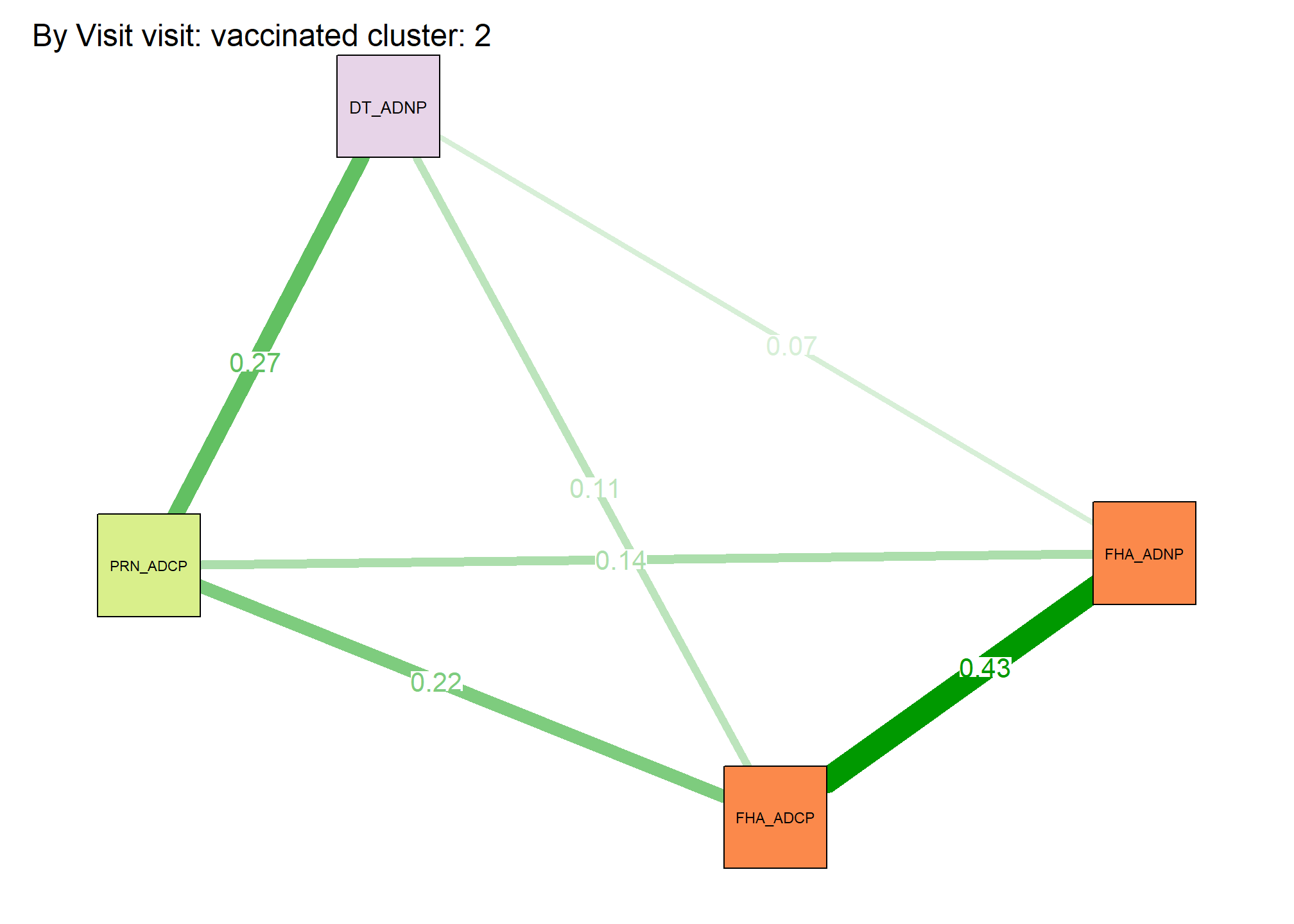 From
To Weight 1 — 2 0.11 1 — 3 0.07 2 — 3 0.43 1 — 4 0.27 2 — 4 0.22 3 — 4
0.14
From
To Weight 1 — 2 0.11 1 — 3 0.07 2 — 3 0.43 1 — 4 0.27 2 — 4 0.22 3 — 4
0.14
Heatmap Subjects Clustered 2
Heatmap Arm Assigned 2
Cluster 3
[1] “DT_FcgR2a” “DT_FcgR3b” “DT_IgG3” “FHA_IgG3” “PRN_IgG3”
“PT_ADCD”
[7] “PT_ADCP” “PT_ADNP” “PT_FcgR2a” “PT_FcgR3b” “PT_IgG1”
“PT_IgG3”
[13] “TT_FcgR2a” “TT_IgG3”
Correlation Heatmap 3
These heatmaps are based on Spearman Rank Correlation.
 [1]
“after cluster specific correlation heatmap”
[1]
“after cluster specific correlation heatmap”
 [1]
“after cluster specific correlation scatter plot grid”
[1]
“after cluster specific correlation scatter plot grid”
Correlation Network 3
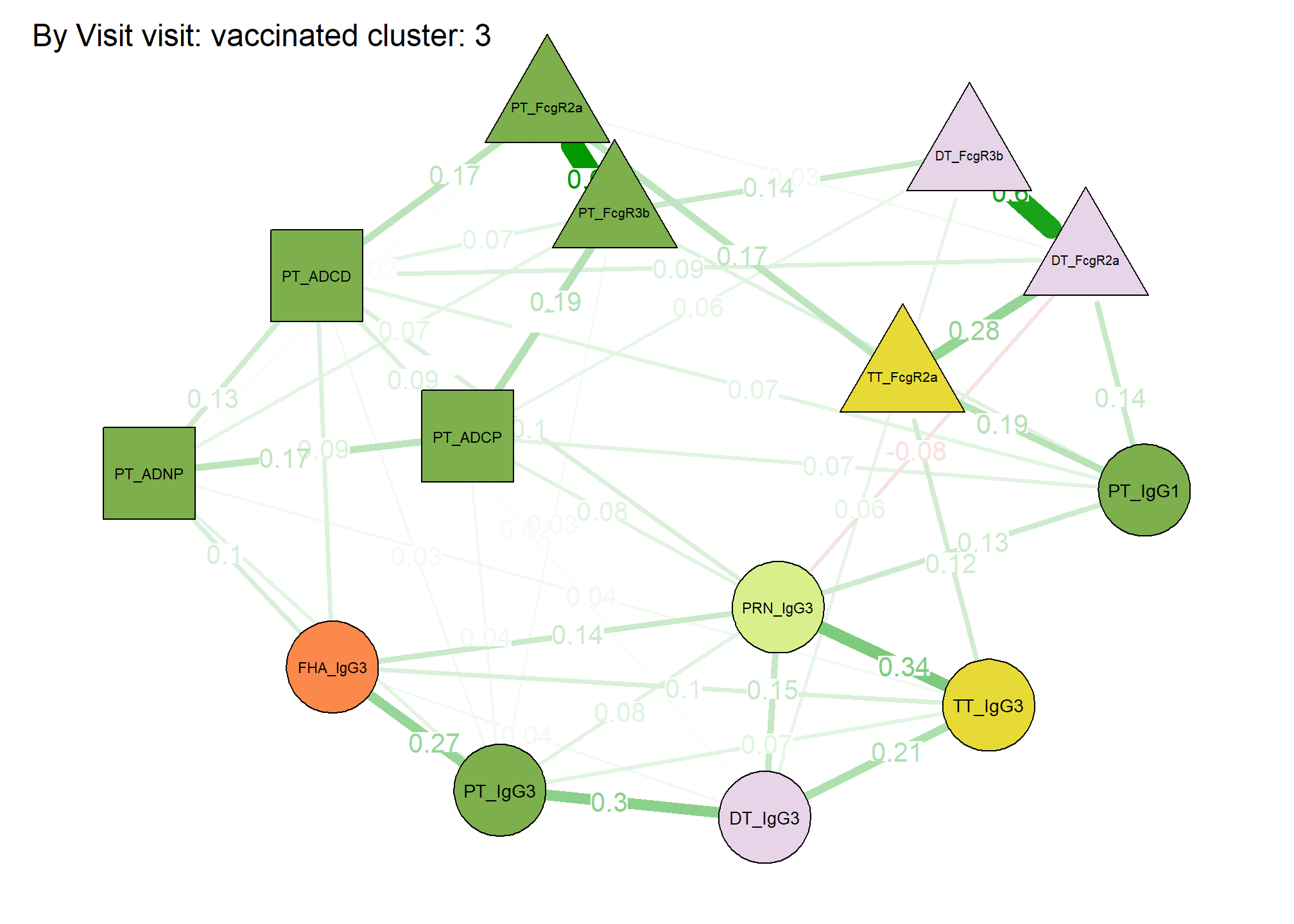
The correlation networks are based on optimal sparse estimates of the partial correlation matrix (Friedman, Hastie and Tibshirani, 2011). Partial correlations represent the remaining association (-1,1) between two nodes after controlling for all other node associations (Epskamp, S. & Fried, Eiko I. (2018)). The lines between nodes are labelled with the partial correlation coefficient. Sometimes there are sparse networks when no significant partial correlation left to plot. Sometimes there are too few samples for the number of features and the correlation matrix becomes indefinite. In either of these circumstances no network plot will be made.
 From
To Weight 1 — 2 0.6 2 — 3 0.06 3 — 4 0.04 1 — 5 -0.08 3 — 5 0.15 4 — 5
0.14 1 — 6 0.09 3 — 6 0.02 4 — 6 0.09 5 — 6 0.1 2 — 7 0.06 5 — 7 0.08 6
— 7 0.09 2 — 8 0.01 4 — 8 0.1 6 — 8 0.13 7 — 8 0.17 1 — 9 0.03 4 — 9
0.01 6 — 9 0.17 8 — 9 0.02 2 — 10 0.14 6 — 10 0.07 7 — 10 0.19 8 — 10
0.07 9 — 10 0.66 1 — 11 0.14 5 — 11 0.13 6 — 11 0.07 7 — 11 0.07 10 — 11
0.09 3 — 12 0.3 4 — 12 0.27 5 — 12 0.08 6 — 12 0.03 7 — 12 0.04 8 — 12
0.07 10 — 12 0.03 1 — 13 0.28 9 — 13 0.17 11 — 13 0.19 3 — 14 0.21 4 —
14 0.1 5 — 14 0.34 8 — 14 0.04 12 — 14 0.07 13 — 14 0.12
From
To Weight 1 — 2 0.6 2 — 3 0.06 3 — 4 0.04 1 — 5 -0.08 3 — 5 0.15 4 — 5
0.14 1 — 6 0.09 3 — 6 0.02 4 — 6 0.09 5 — 6 0.1 2 — 7 0.06 5 — 7 0.08 6
— 7 0.09 2 — 8 0.01 4 — 8 0.1 6 — 8 0.13 7 — 8 0.17 1 — 9 0.03 4 — 9
0.01 6 — 9 0.17 8 — 9 0.02 2 — 10 0.14 6 — 10 0.07 7 — 10 0.19 8 — 10
0.07 9 — 10 0.66 1 — 11 0.14 5 — 11 0.13 6 — 11 0.07 7 — 11 0.07 10 — 11
0.09 3 — 12 0.3 4 — 12 0.27 5 — 12 0.08 6 — 12 0.03 7 — 12 0.04 8 — 12
0.07 10 — 12 0.03 1 — 13 0.28 9 — 13 0.17 11 — 13 0.19 3 — 14 0.21 4 —
14 0.1 5 — 14 0.34 8 — 14 0.04 12 — 14 0.07 13 — 14 0.12
Heatmap Subjects Clustered 3
Heatmap Arm Assigned 3
Cluster 4
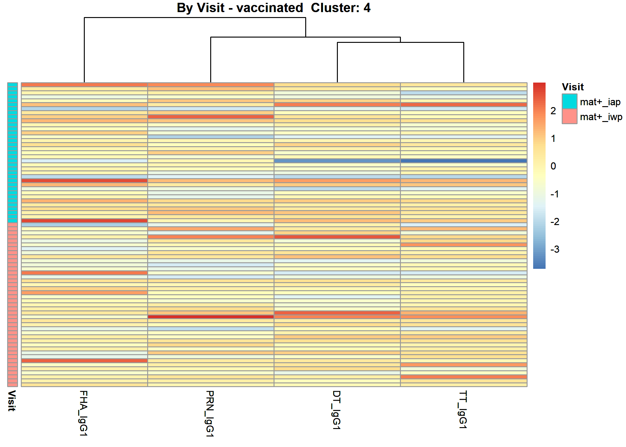
[1] “DT_IgG1” “FHA_IgG1” “PRN_IgG1” “TT_IgG1”
Correlation Heatmap 4
These heatmaps are based on Spearman Rank Correlation.
 [1]
“after cluster specific correlation heatmap”
[1]
“after cluster specific correlation heatmap”
 [1]
“after cluster specific correlation scatter plot grid”
[1]
“after cluster specific correlation scatter plot grid”
Correlation Network 4
The correlation networks are based on optimal sparse estimates of the partial correlation matrix (Friedman, Hastie and Tibshirani, 2011). Partial correlations represent the remaining association (-1,1) between two nodes after controlling for all other node associations (Epskamp, S. & Fried, Eiko I. (2018)). The lines between nodes are labelled with the partial correlation coefficient. Sometimes there are sparse networks when no significant partial correlation left to plot. Sometimes there are too few samples for the number of features and the correlation matrix becomes indefinite. In either of these circumstances no network plot will be made.
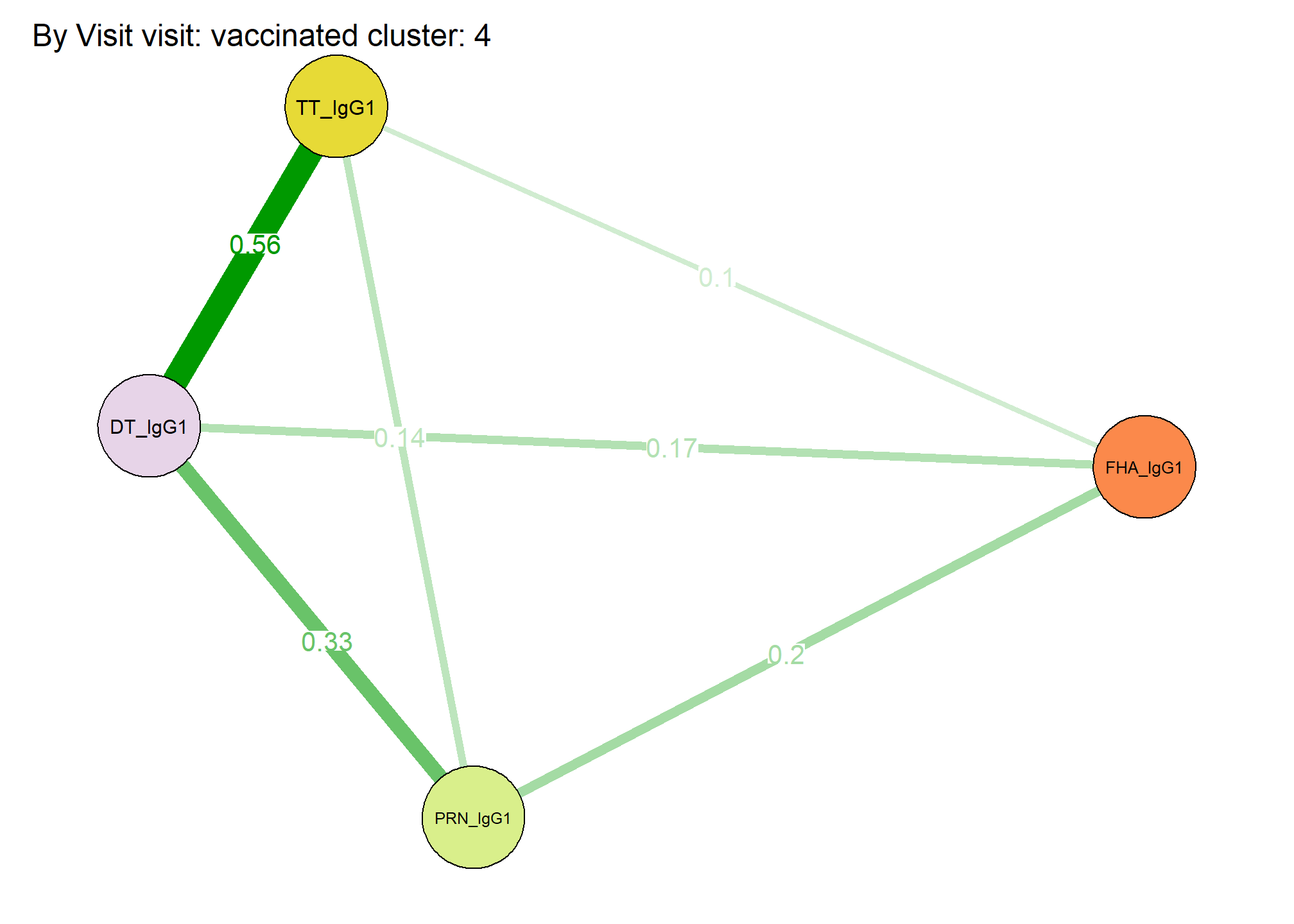 From
To Weight 1 — 2 0.17 1 — 3 0.33 2 — 3 0.2 1 — 4 0.56 2 — 4 0.1 3 — 4
0.14
From
To Weight 1 — 2 0.17 1 — 3 0.33 2 — 3 0.2 1 — 4 0.56 2 — 4 0.1 3 — 4
0.14
Heatmap Subjects Clustered 4
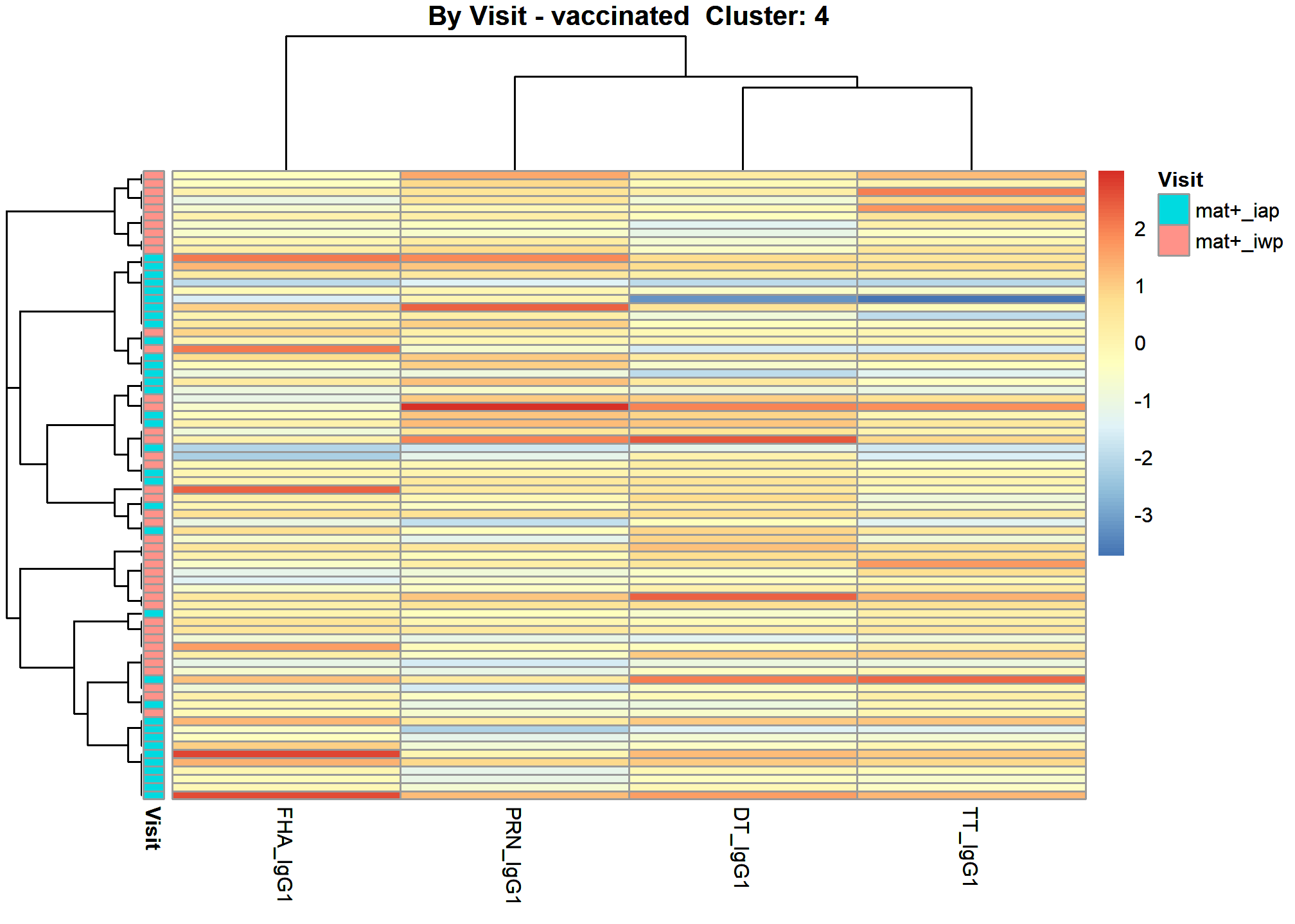
Heatmap Arm Assigned 4
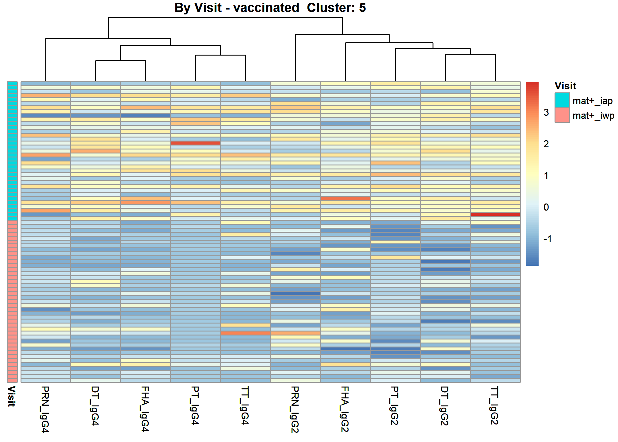
Cluster 5
[1] “DT_IgG2” “DT_IgG4” “FHA_IgG2” “FHA_IgG4” “PRN_IgG2” “PRN_IgG4” [7] “PT_IgG2” “PT_IgG4” “TT_IgG2” “TT_IgG4”
Correlation Heatmap 5
These heatmaps are based on Spearman Rank Correlation.
 [1]
“after cluster specific correlation heatmap”
[1]
“after cluster specific correlation heatmap”
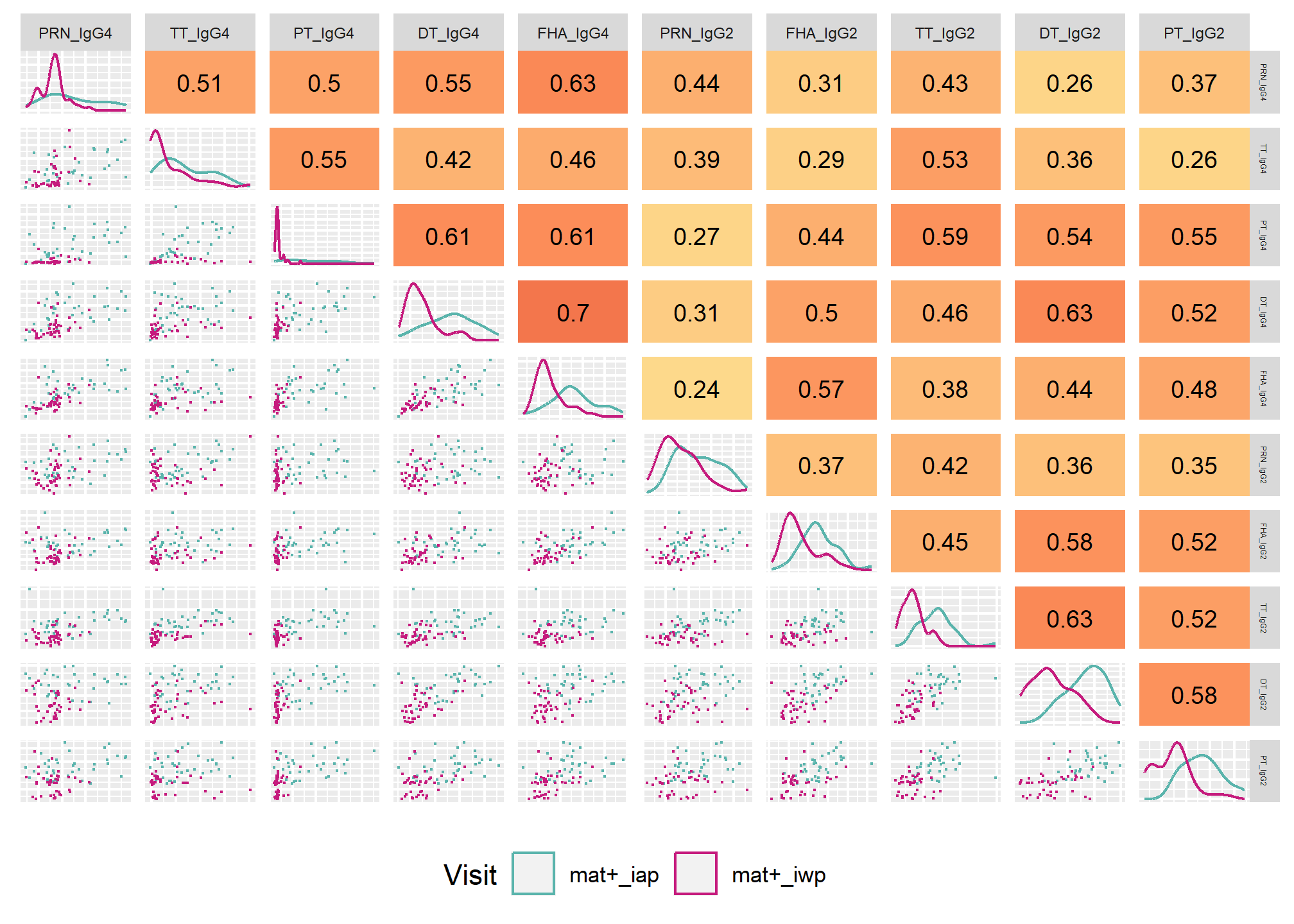 [1]
“after cluster specific correlation scatter plot grid”
[1]
“after cluster specific correlation scatter plot grid”
Correlation Network 5
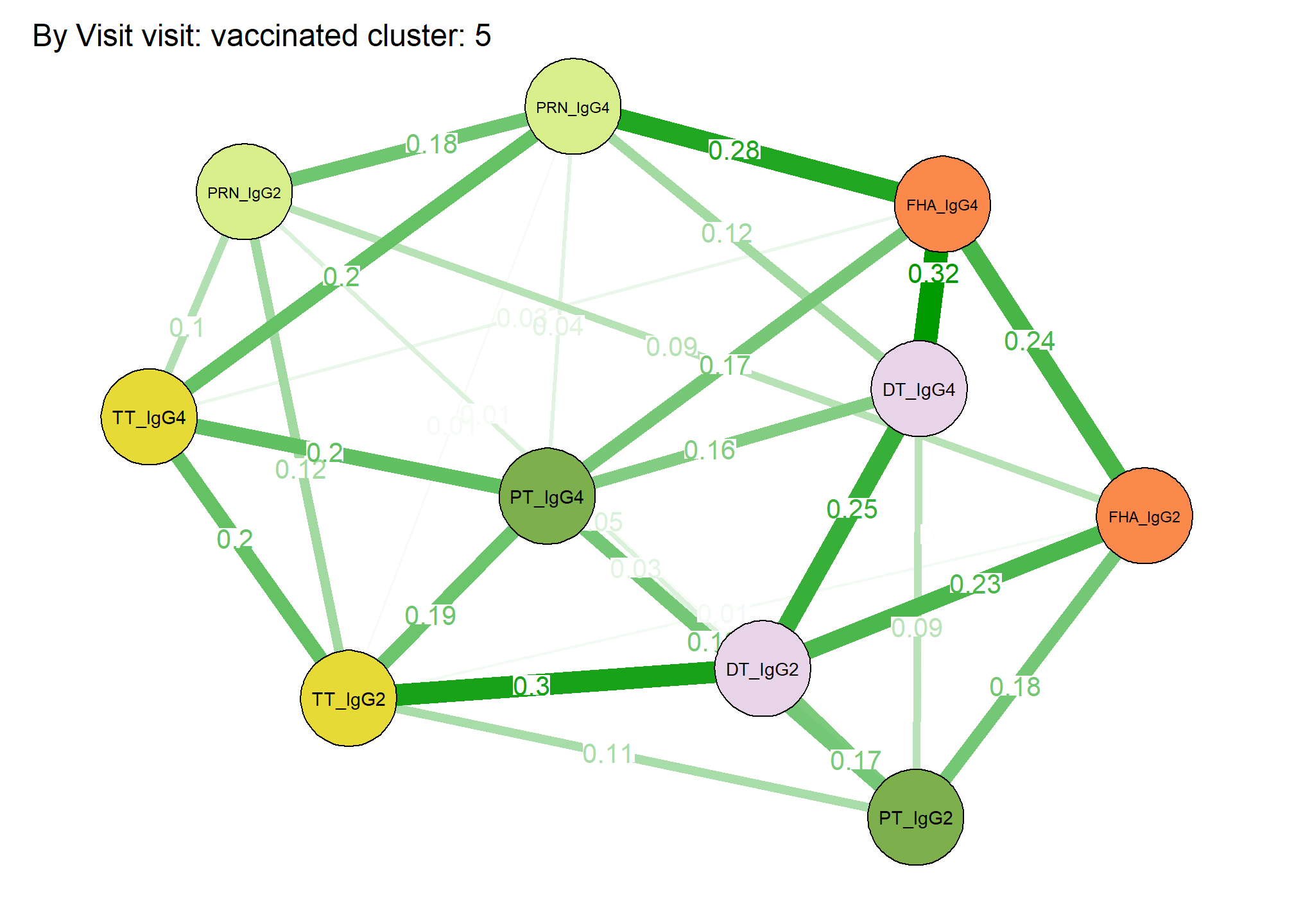
The correlation networks are based on optimal sparse estimates of the partial correlation matrix (Friedman, Hastie and Tibshirani, 2011). Partial correlations represent the remaining association (-1,1) between two nodes after controlling for all other node associations (Epskamp, S. & Fried, Eiko I. (2018)). The lines between nodes are labelled with the partial correlation coefficient. Sometimes there are sparse networks when no significant partial correlation left to plot. Sometimes there are too few samples for the number of features and the correlation matrix becomes indefinite. In either of these circumstances no network plot will be made.
 From
To Weight 1 — 2 0.25 1 — 3 0.23 2 — 4 0.32 3 — 4 0.24 1 — 5 0.01 3 — 5
0.09 2 — 6 0.12 4 — 6 0.28 5 — 6 0.18 1 — 7 0.17 2 — 7 0.09 3 — 7 0.18 4
— 7 0 5 — 7 0.05 1 — 8 0.03 2 — 8 0.16 4 — 8 0.17 6 — 8 0.04 7 — 8 0.18
1 — 9 0.3 3 — 9 0.01 5 — 9 0.12 6 — 9 0.01 7 — 9 0.11 8 — 9 0.19 4 — 10
0.03 5 — 10 0.1 6 — 10 0.2 8 — 10 0.2 9 — 10 0.2
From
To Weight 1 — 2 0.25 1 — 3 0.23 2 — 4 0.32 3 — 4 0.24 1 — 5 0.01 3 — 5
0.09 2 — 6 0.12 4 — 6 0.28 5 — 6 0.18 1 — 7 0.17 2 — 7 0.09 3 — 7 0.18 4
— 7 0 5 — 7 0.05 1 — 8 0.03 2 — 8 0.16 4 — 8 0.17 6 — 8 0.04 7 — 8 0.18
1 — 9 0.3 3 — 9 0.01 5 — 9 0.12 6 — 9 0.01 7 — 9 0.11 8 — 9 0.19 4 — 10
0.03 5 — 10 0.1 6 — 10 0.2 8 — 10 0.2 9 — 10 0.2
Heatmap Subjects Clustered 5
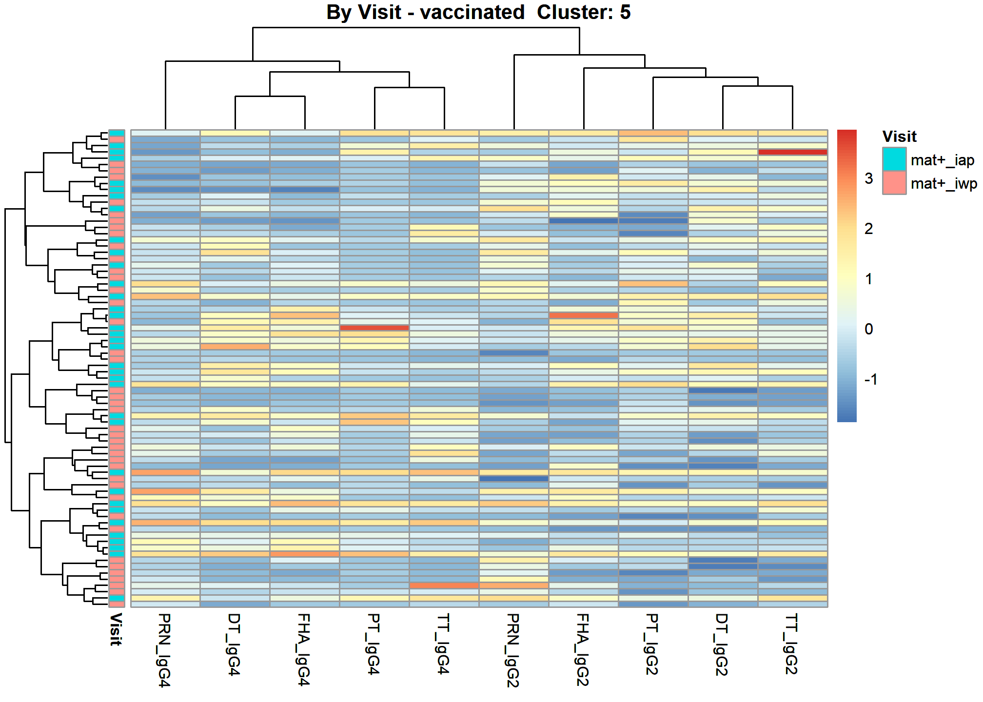
Heatmap Arm Assigned 5
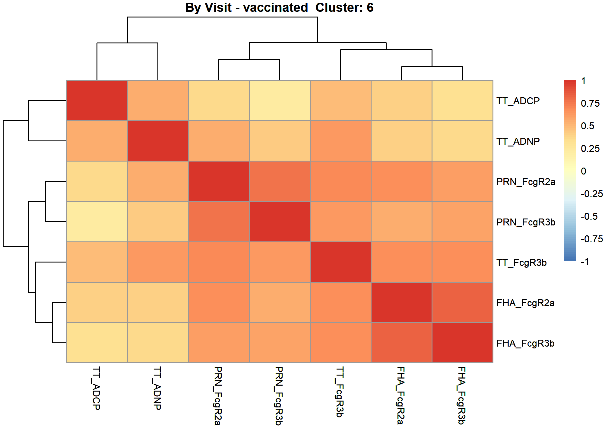
Cluster 6
[1] “FHA_FcgR2a” “FHA_FcgR3b” “PRN_FcgR2a” “PRN_FcgR3b”
“TT_ADCP”
[6] “TT_ADNP” “TT_FcgR3b”
Correlation Heatmap 6
These heatmaps are based on Spearman Rank Correlation.
 [1]
“after cluster specific correlation heatmap”
[1]
“after cluster specific correlation heatmap”
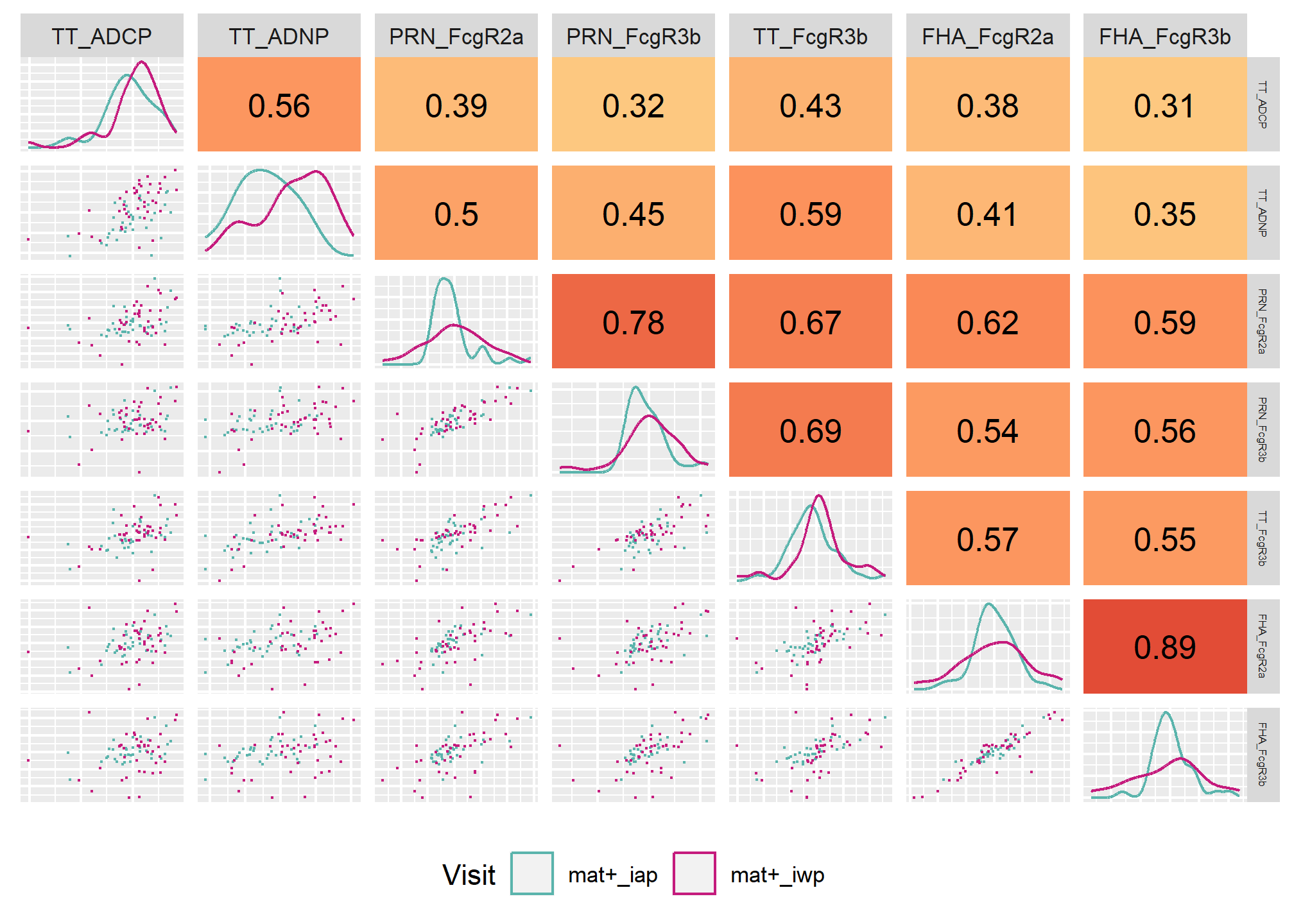 [1]
“after cluster specific correlation scatter plot grid”
[1]
“after cluster specific correlation scatter plot grid”
Correlation Network 6
The correlation networks are based on optimal sparse estimates of the partial correlation matrix (Friedman, Hastie and Tibshirani, 2011). Partial correlations represent the remaining association (-1,1) between two nodes after controlling for all other node associations (Epskamp, S. & Fried, Eiko I. (2018)). The lines between nodes are labelled with the partial correlation coefficient. Sometimes there are sparse networks when no significant partial correlation left to plot. Sometimes there are too few samples for the number of features and the correlation matrix becomes indefinite. In either of these circumstances no network plot will be made.
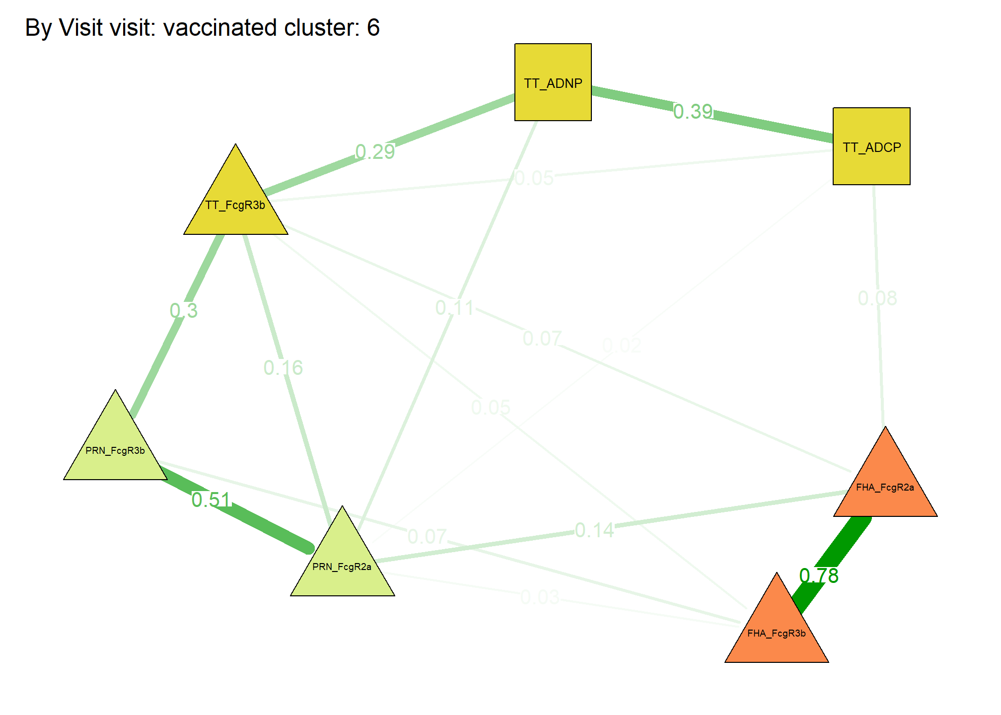 From
To Weight 1 — 2 0.78 1 — 3 0.14 2 — 3 0.03 2 — 4 0.07 3 — 4 0.51 1 — 5
0.08 3 — 5 0.02 3 — 6 0.11 5 — 6 0.39 1 — 7 0.07 2 — 7 0.05 3 — 7 0.16 4
— 7 0.3 5 — 7 0.05 6 — 7 0.29
From
To Weight 1 — 2 0.78 1 — 3 0.14 2 — 3 0.03 2 — 4 0.07 3 — 4 0.51 1 — 5
0.08 3 — 5 0.02 3 — 6 0.11 5 — 6 0.39 1 — 7 0.07 2 — 7 0.05 3 — 7 0.16 4
— 7 0.3 5 — 7 0.05 6 — 7 0.29
Heatmap Subjects Clustered 6
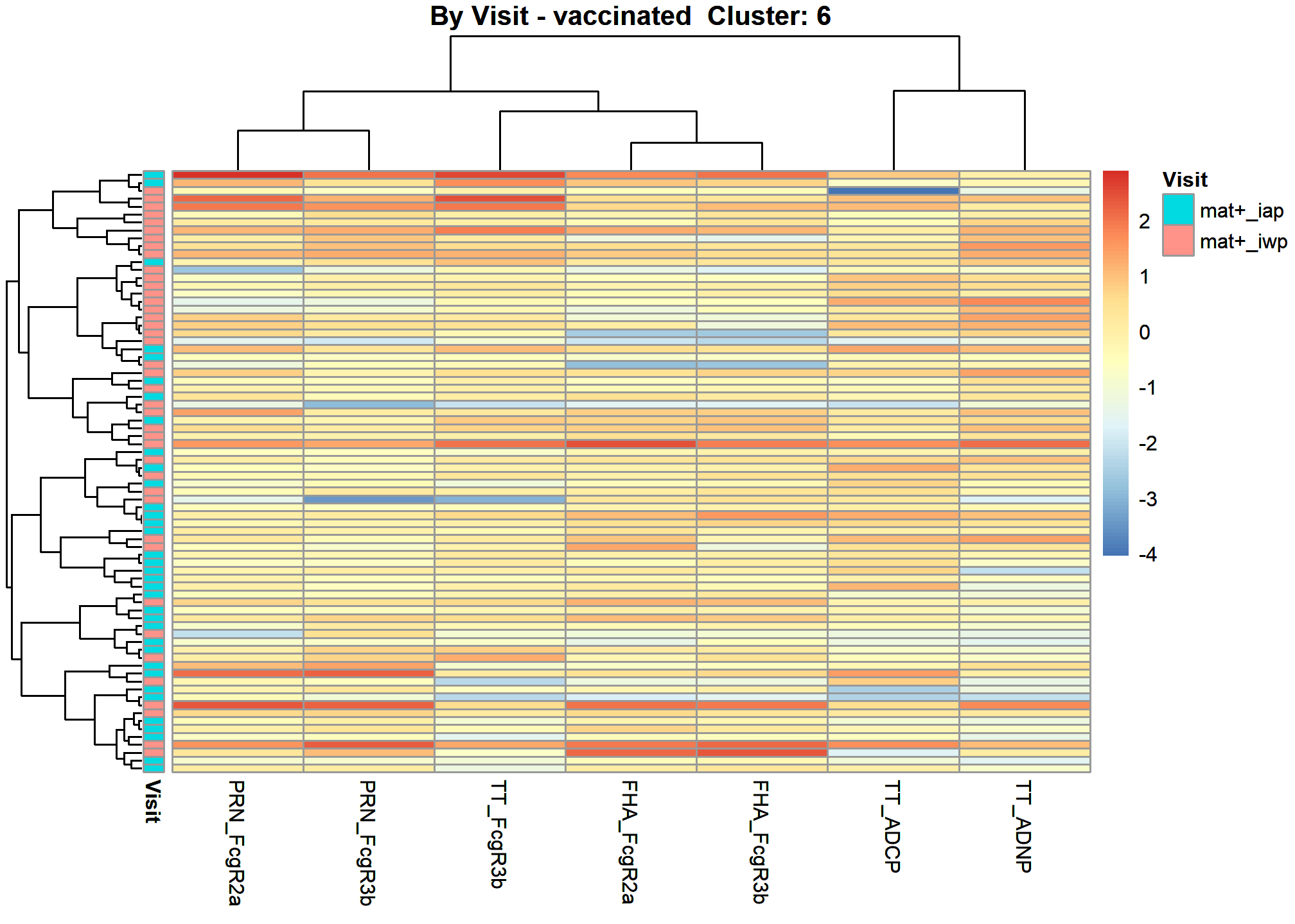
Heatmap Arm Assigned 6
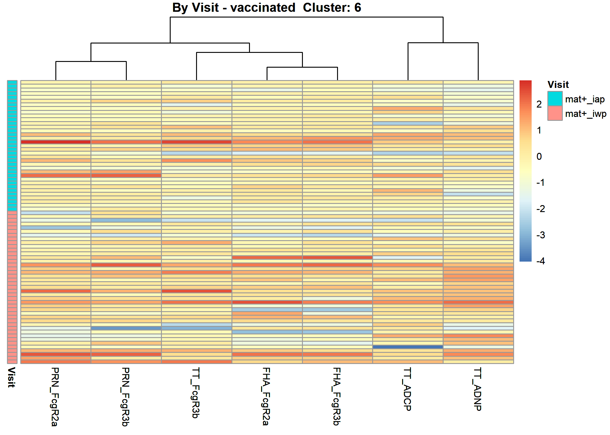
By Visit - boosted : Results
Heatmap clustering
Cluster Arms

[1] “after_cluster_arms”
Fix Arms
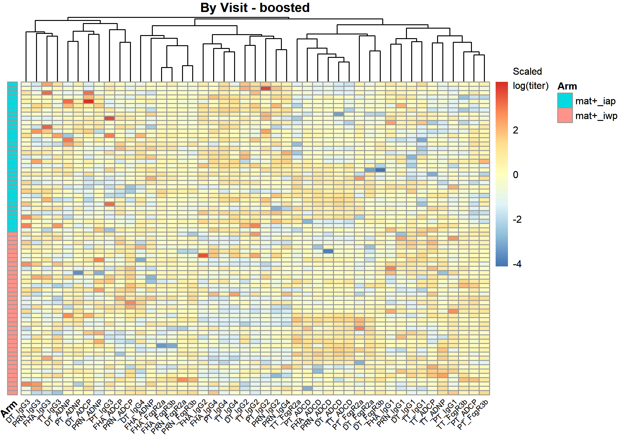
[1] “after_fix_arms”
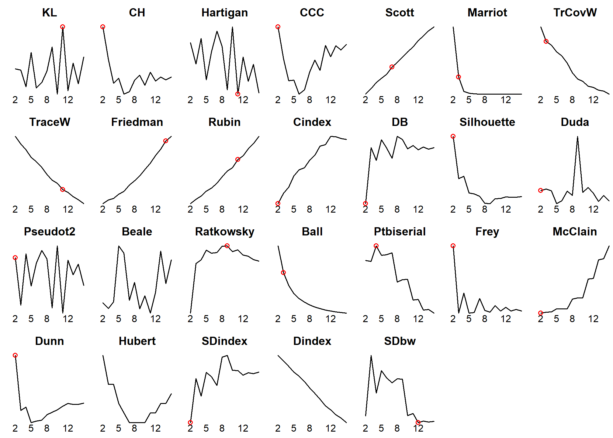
Number of Clusters
Among all indices:
11 proposed 2 as the best number of clusters
3 proposed 3 as the best number of clusters
1 proposed 4 as the best number of clusters
1 proposed 7 as the best number of clusters
1 proposed 9 as the best number of clusters
4 proposed 11 as the best number of clusters
1 proposed 12 as the best number of clusters
1 proposed 14 as the best number of clusters
1 proposed 15 as the best number of clusters
***** Conclusion *****According to the majority rule, the best number of clusters is 2
Dendrogram
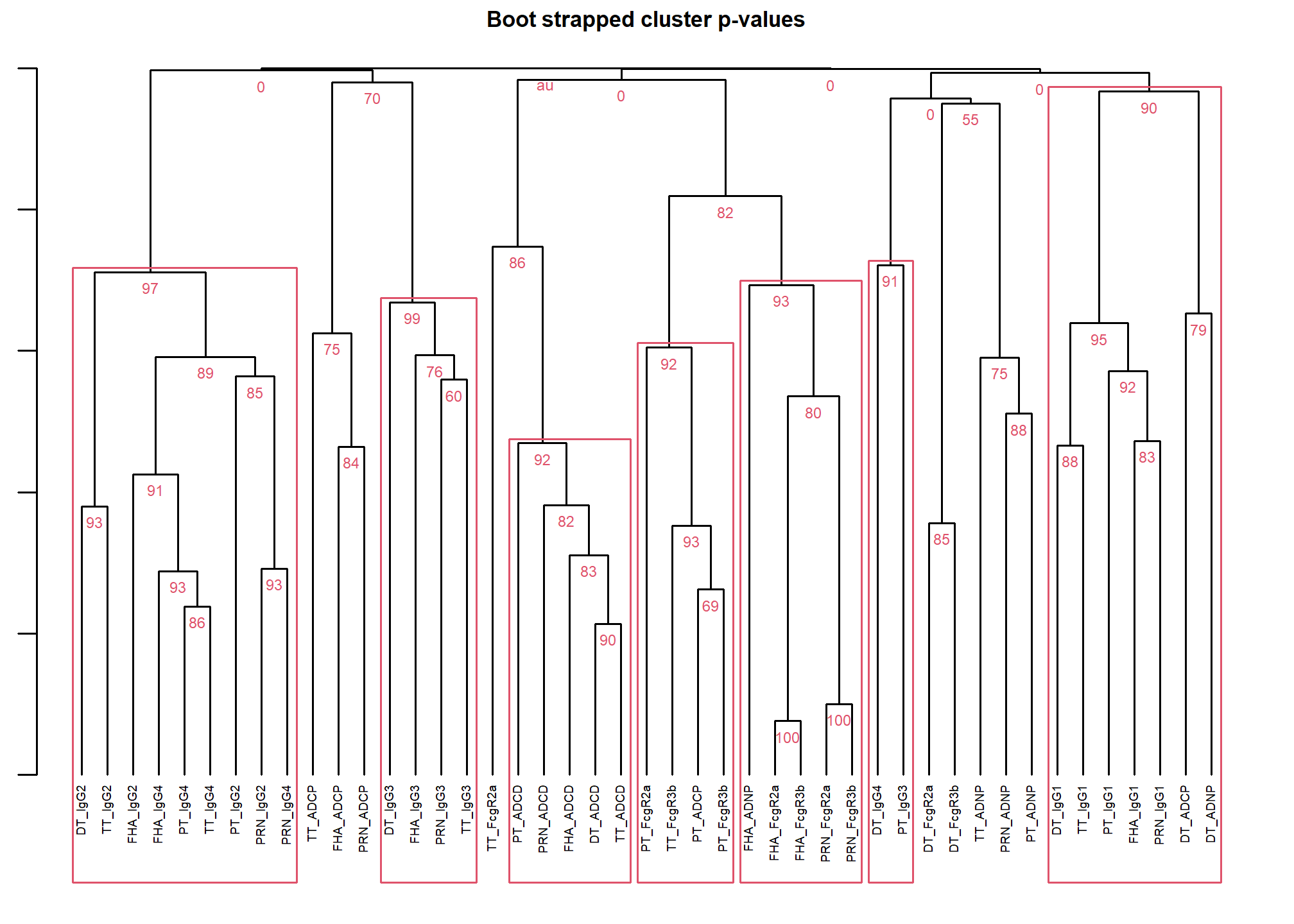
Whole feature set clustering: basic clusters and tree branch boot strap tests
[1] “after_dendrogram”
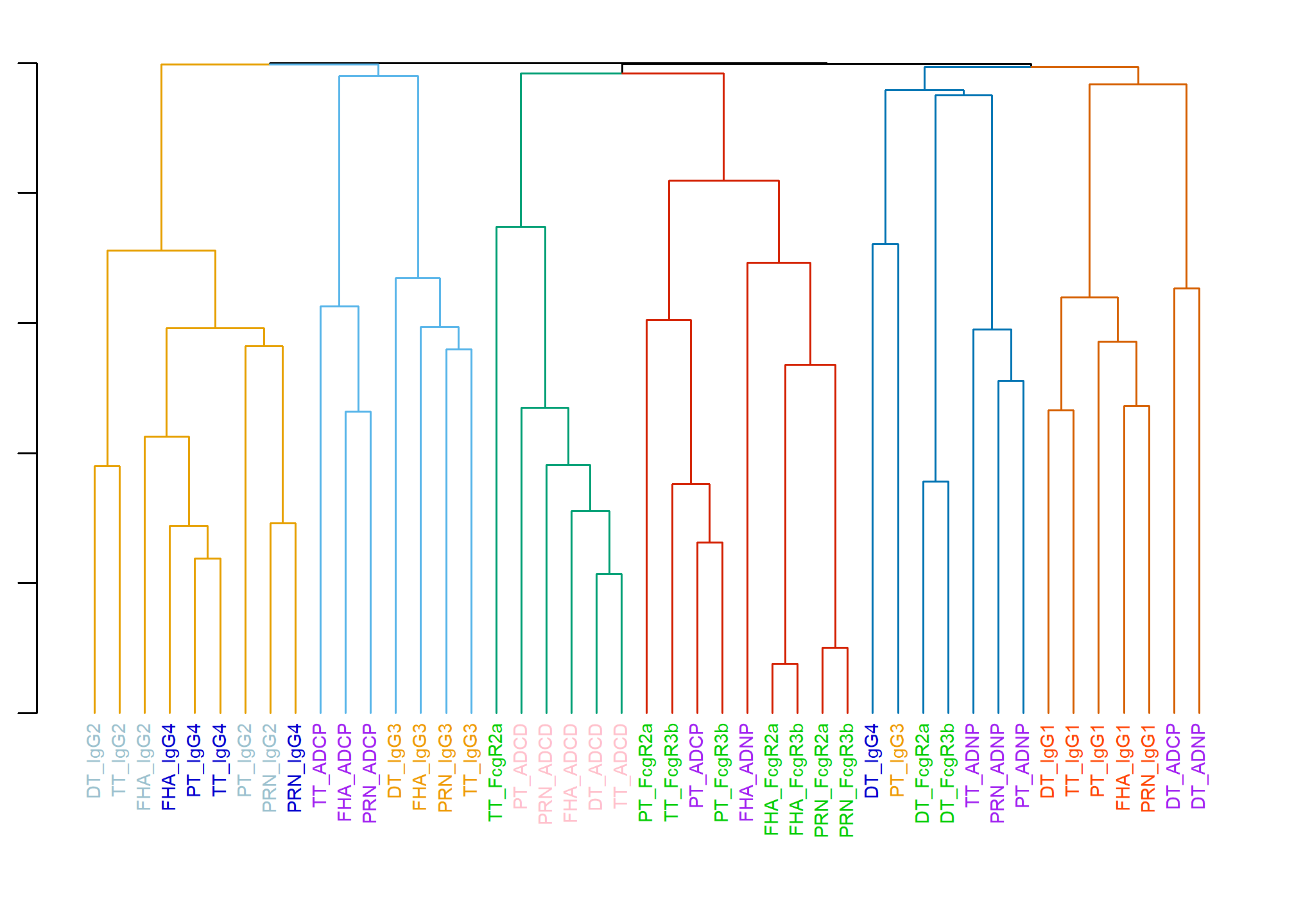
Hierarchical Clusters
The number of clusters shown is optimized using the preponderance of indicies for this purpose.
[1] “after_dendlistnew”
Tree Branch Tests
References
Suzuki, R. and Shimodaira, H. (2006) Pvclust: an R package for assessing the uncertainty in hierarchical clustering, Bioinformatics, 22 (12): 1540-1542.
Shimodaira, H. (2004) Approximately unbiased tests of regions using multistep-multiscale bootstrap resampling, Annals of Statistics, 32, 2616-2641.
Shimodaira, H. (2002) An approximately unbiased test of phylogenetic tree selection, Systematic Biology, 51, 492-508.
Suzuki, R. and Shimodaira, H. (2004) An application of multiscale bootstrap resampling to hierarchical clustering of microarray data: How accurate are these clusters?, The Fifteenth International Conference on Genome Informatics 2004, P034.
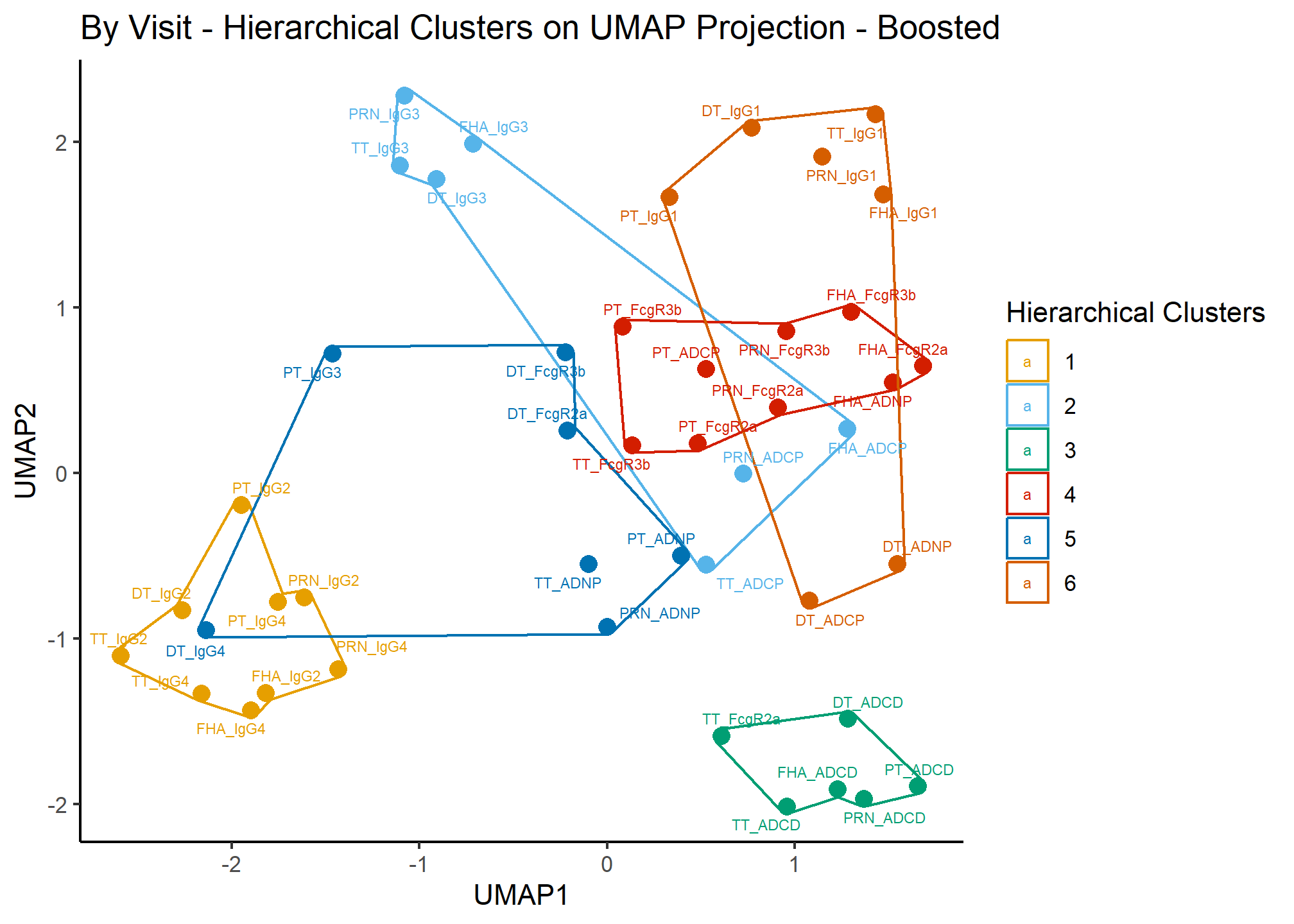
UMAP Concordance
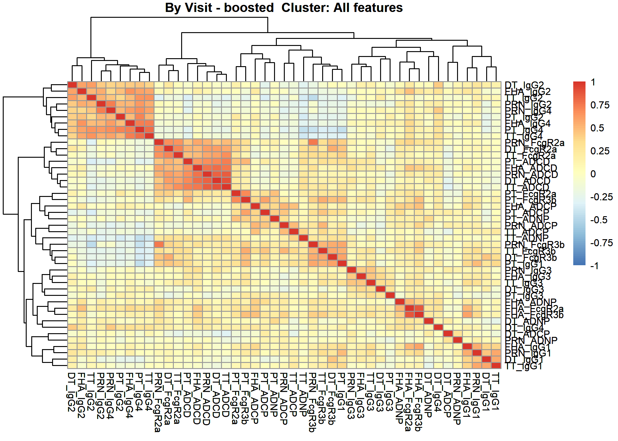
Correlation Heatmap: all features
These heatmaps are based on Spearman Rank Correlation.
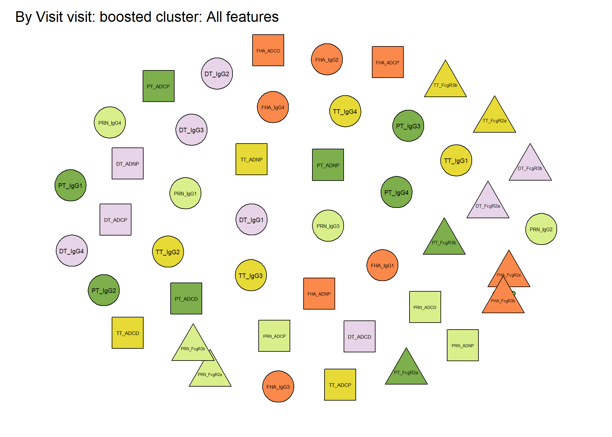
Correlation Network: all features
The correlation networks are based on Partial Correlation. This means that all the correlation between pairs of features after all the other correlation is accounted for. Sometimes there are sparse networks when no significant partial correlation left to plot. Sometimes there are too few samples for the number of features and the correlation matrix becomes indefinite. In either of these circumstances no network plot will be made.
 From
To Weight 13 — 14 0.12 22 — 23 0.1
From
To Weight 13 — 14 0.12 22 — 23 0.1
Cluster Contents
| name | contents |
|---|---|
| Cluster_1 | DT_ADCD, FHA_ADCD, PRN_ADCD, PT_ADCD, TT_ADCD, TT_FcgR2a |
| Cluster_2 | DT_ADCP, DT_ADNP, DT_IgG1, FHA_IgG1, PRN_IgG1, PT_IgG1, TT_IgG1 |
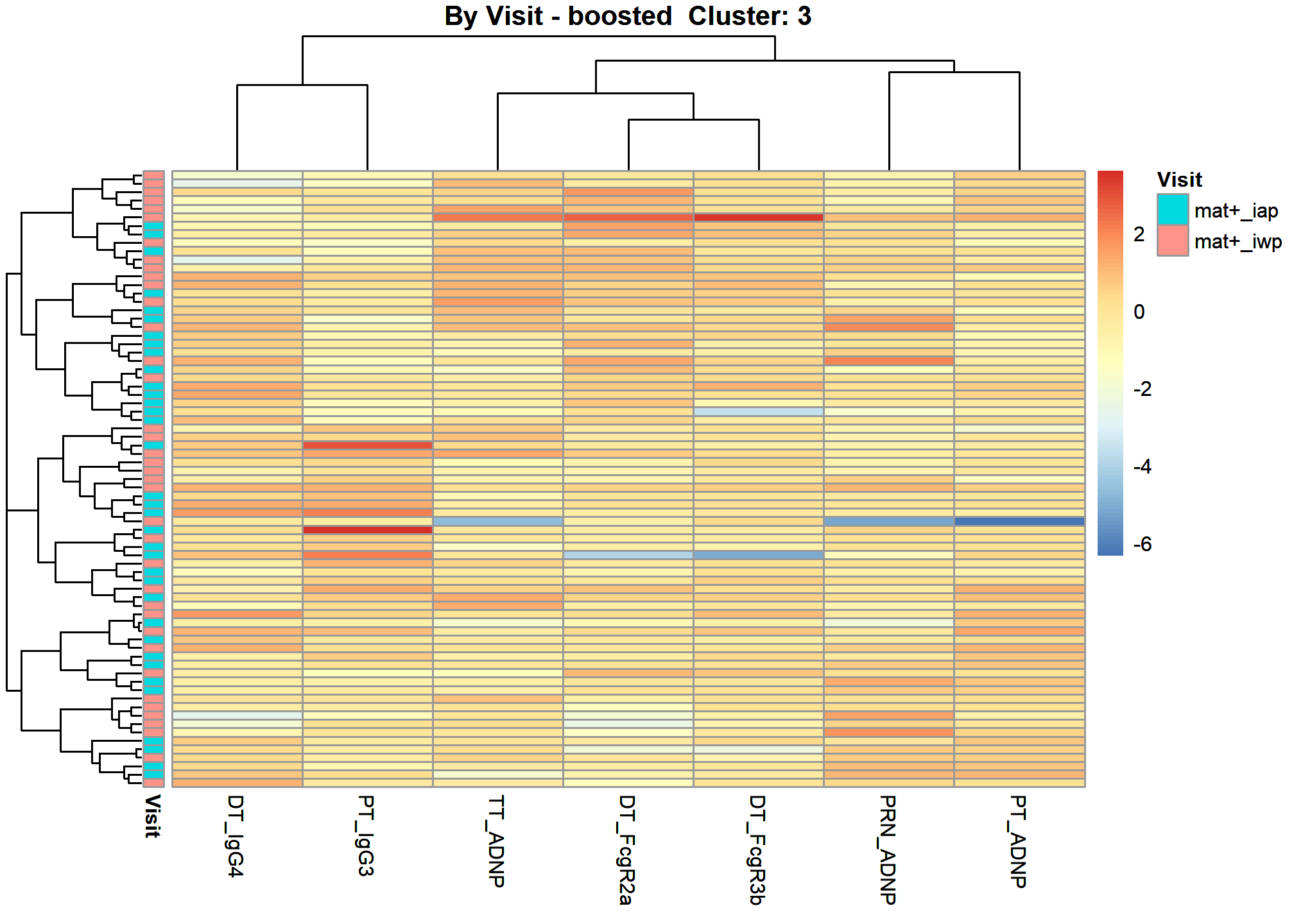
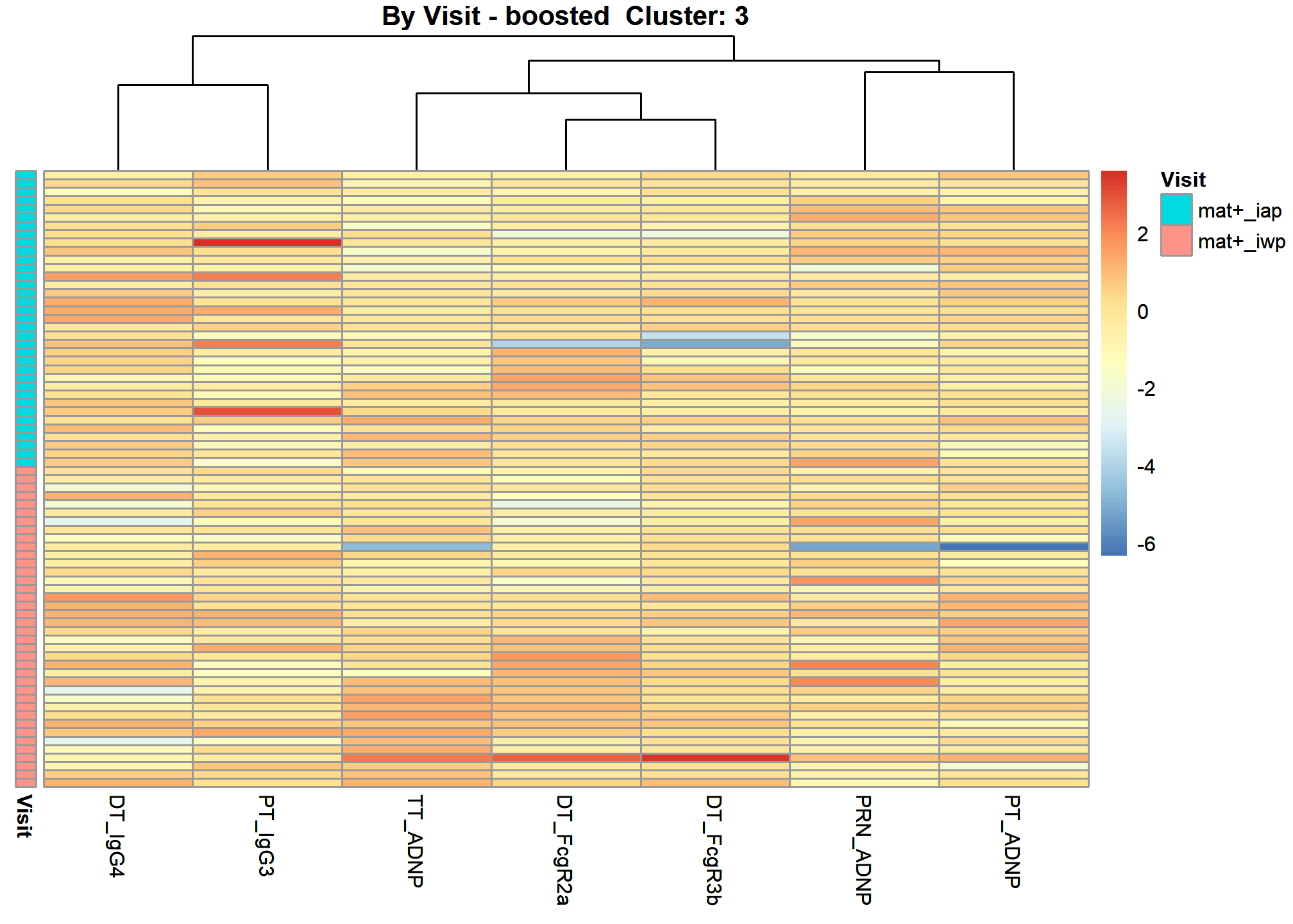
| Cluster_3 | DT_FcgR2a, DT_FcgR3b, DT_IgG4, PRN_ADNP, PT_ADNP, PT_IgG3, TT_ADNP |
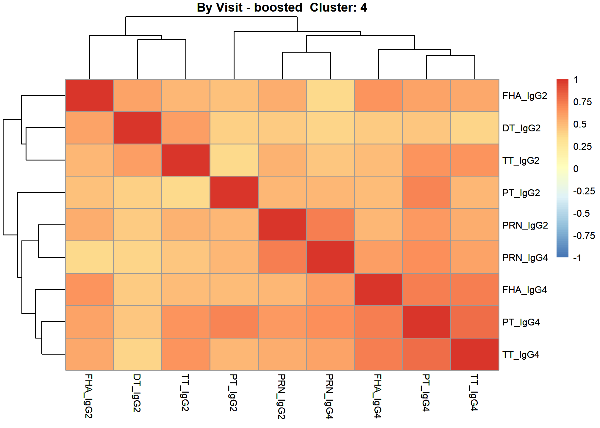
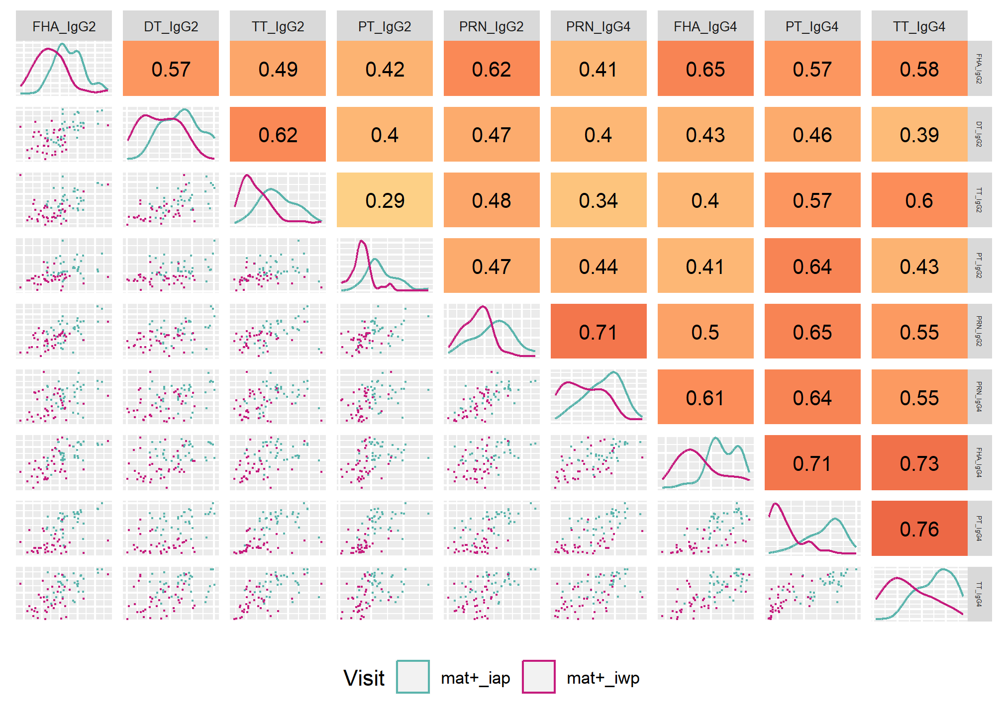
| Cluster_4 | DT_IgG2, FHA_IgG2, FHA_IgG4, PRN_IgG2, PRN_IgG4, PT_IgG2, PT_IgG4, TT_IgG2, TT_IgG4 |
| Cluster_5 | DT_IgG3, FHA_ADCP, FHA_IgG3, PRN_ADCP, PRN_IgG3, TT_ADCP, TT_IgG3 |
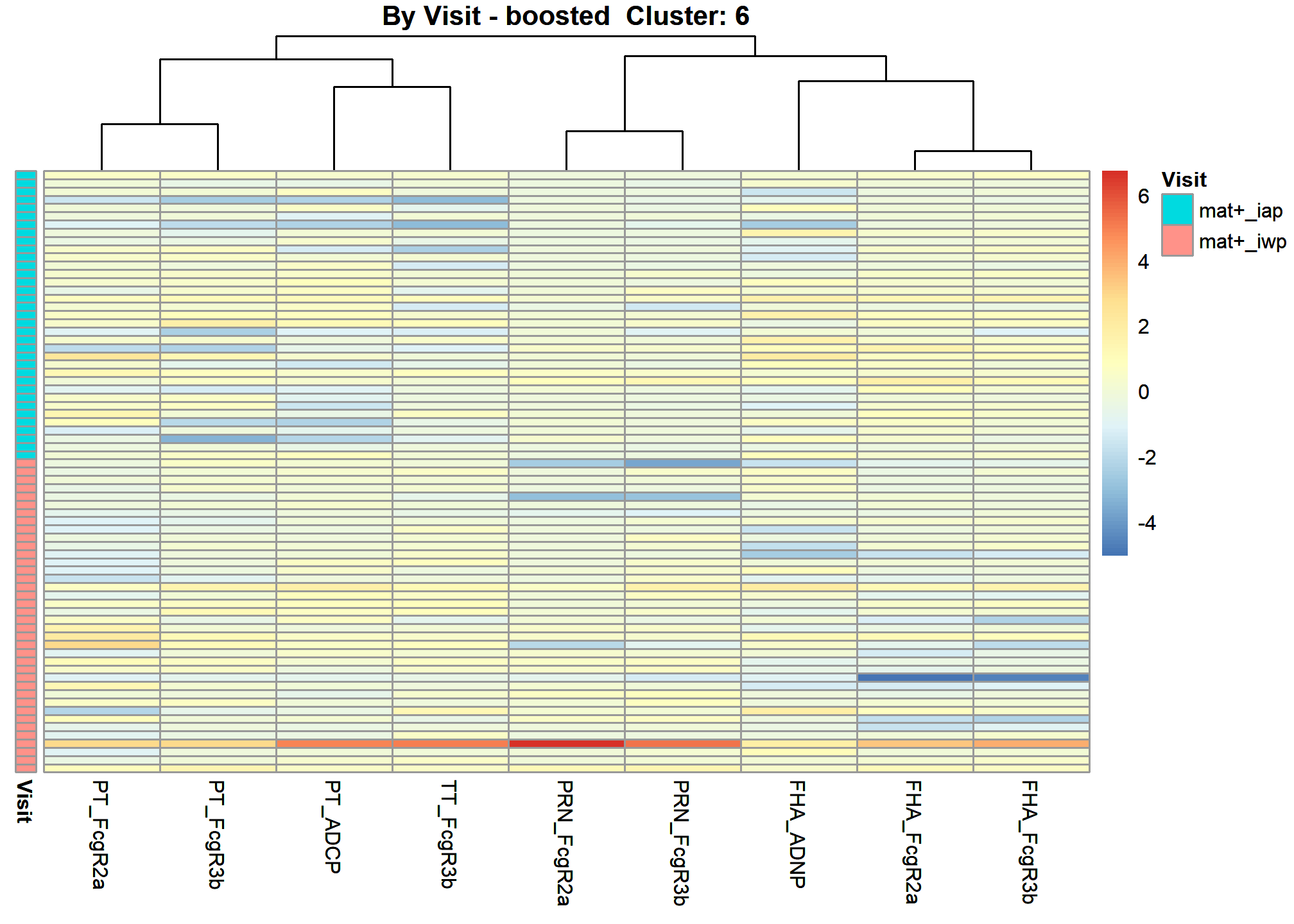
| Cluster_6 | FHA_ADNP, FHA_FcgR2a, FHA_FcgR3b, PRN_FcgR2a, PRN_FcgR3b, PT_ADCP, PT_FcgR2a, PT_FcgR3b, TT_FcgR3b |
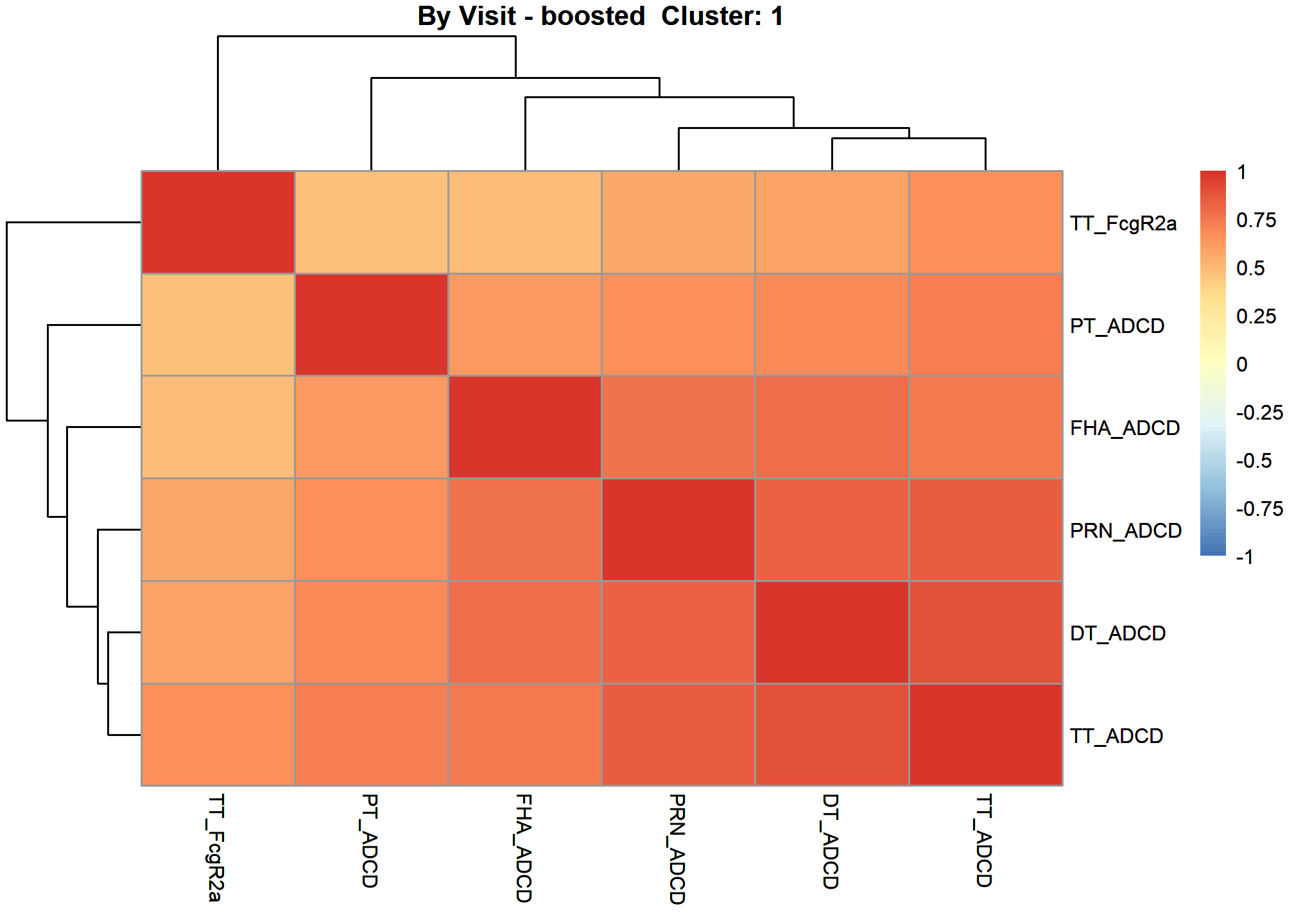
Cluster 1
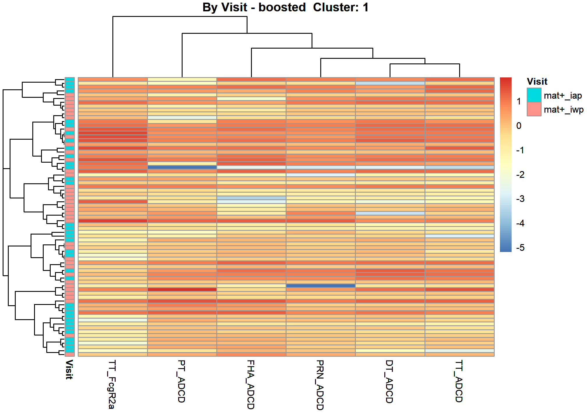
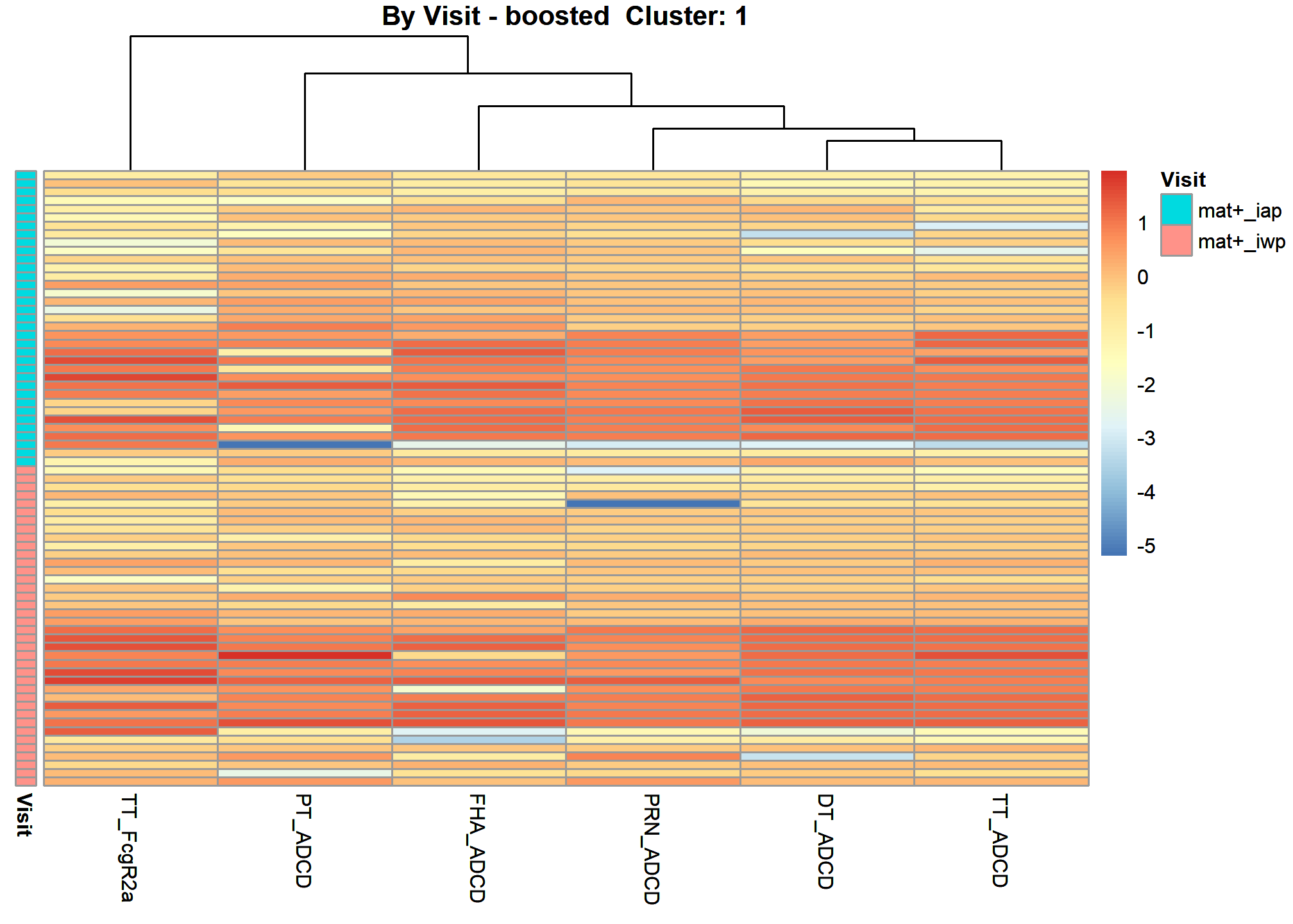
[1] “DT_ADCD” “FHA_ADCD” “PRN_ADCD” “PT_ADCD” “TT_ADCD” “TT_FcgR2a”
Correlation Heatmap 1
These heatmaps are based on Spearman Rank Correlation.
 [1]
“after cluster specific correlation heatmap”
[1]
“after cluster specific correlation heatmap”
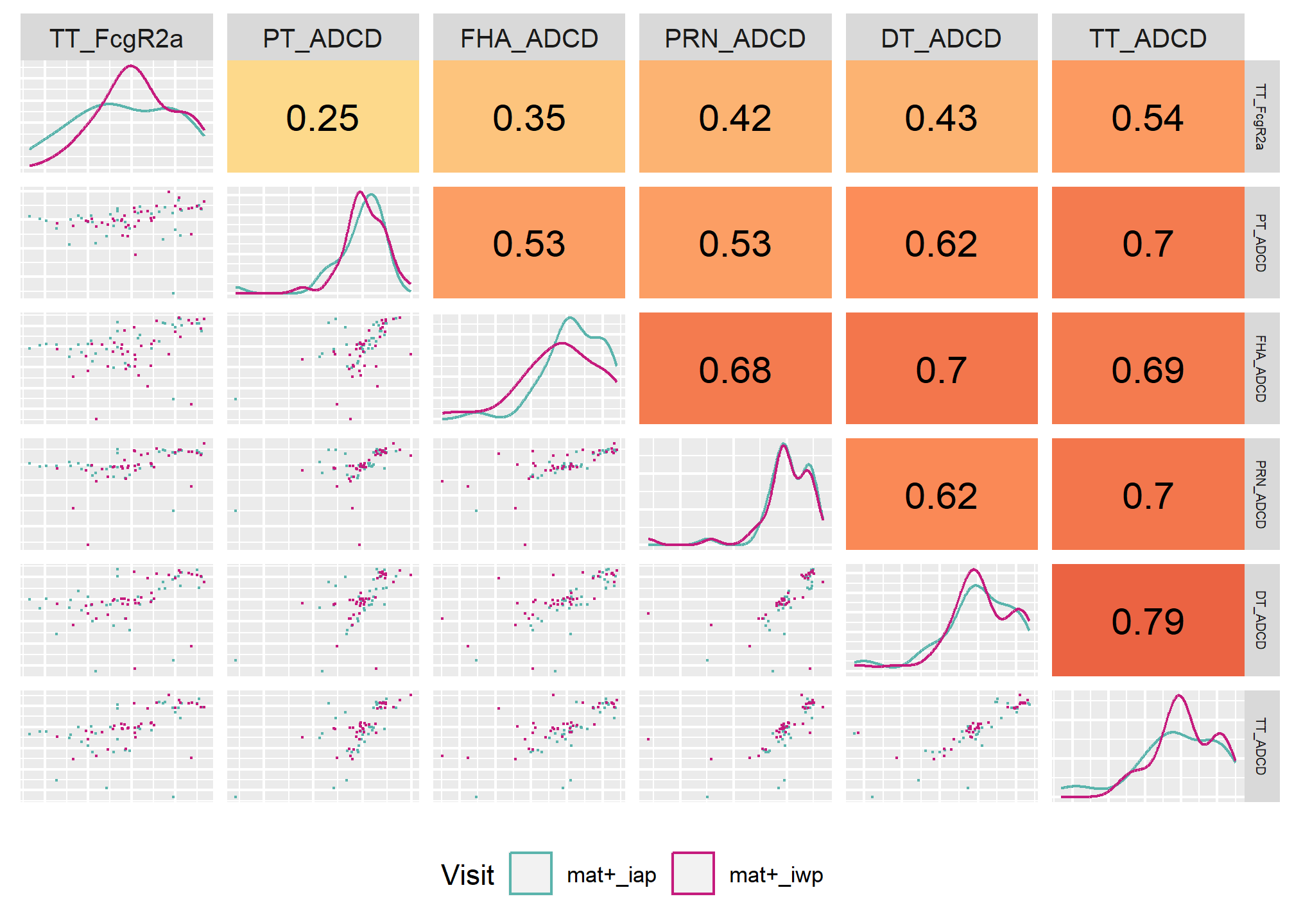 [1]
“after cluster specific correlation scatter plot grid”
[1]
“after cluster specific correlation scatter plot grid”
Correlation Network 1
The correlation networks are based on optimal sparse estimates of the partial correlation matrix (Friedman, Hastie and Tibshirani, 2011). Partial correlations represent the remaining association (-1,1) between two nodes after controlling for all other node associations (Epskamp, S. & Fried, Eiko I. (2018)). The lines between nodes are labelled with the partial correlation coefficient. Sometimes there are sparse networks when no significant partial correlation left to plot. Sometimes there are too few samples for the number of features and the correlation matrix becomes indefinite. In either of these circumstances no network plot will be made.
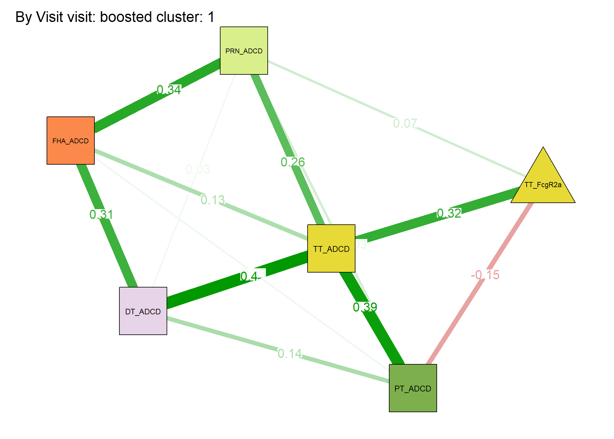 From
To Weight 1 — 2 0.31 1 — 3 0.03 2 — 3 0.34 1 — 4 0.14 2 — 4 0.03 3 — 4
0.07 1 — 5 0.4 2 — 5 0.13 3 — 5 0.26 4 — 5 0.39 1 — 6 0.03 3 — 6 0.07 4
— 6 -0.15 5 — 6 0.32
From
To Weight 1 — 2 0.31 1 — 3 0.03 2 — 3 0.34 1 — 4 0.14 2 — 4 0.03 3 — 4
0.07 1 — 5 0.4 2 — 5 0.13 3 — 5 0.26 4 — 5 0.39 1 — 6 0.03 3 — 6 0.07 4
— 6 -0.15 5 — 6 0.32
Heatmap Subjects Clustered 1
Heatmap Arm Assigned 1
Cluster 2
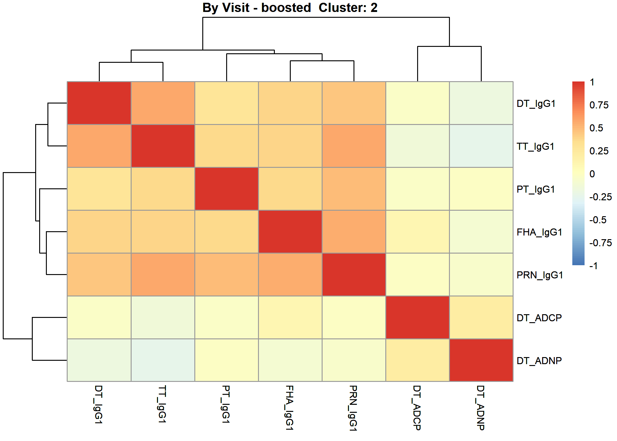
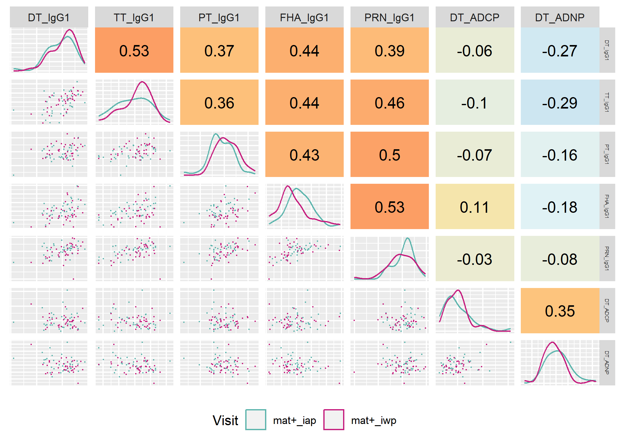
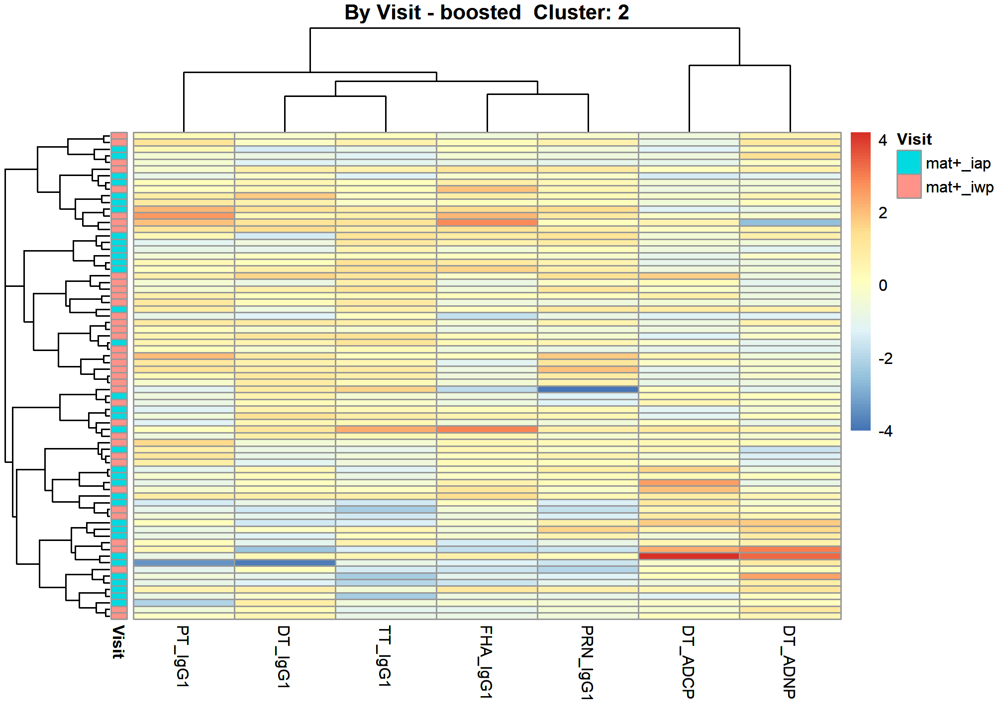
[1] “DT_ADCP” “DT_ADNP” “DT_IgG1” “FHA_IgG1” “PRN_IgG1” “PT_IgG1” “TT_IgG1”
Correlation Heatmap 2
These heatmaps are based on Spearman Rank Correlation.
 [1]
“after cluster specific correlation heatmap”
[1]
“after cluster specific correlation heatmap”
 [1]
“after cluster specific correlation scatter plot grid”
[1]
“after cluster specific correlation scatter plot grid”
Correlation Network 2
The correlation networks are based on optimal sparse estimates of the partial correlation matrix (Friedman, Hastie and Tibshirani, 2011). Partial correlations represent the remaining association (-1,1) between two nodes after controlling for all other node associations (Epskamp, S. & Fried, Eiko I. (2018)). The lines between nodes are labelled with the partial correlation coefficient. Sometimes there are sparse networks when no significant partial correlation left to plot. Sometimes there are too few samples for the number of features and the correlation matrix becomes indefinite. In either of these circumstances no network plot will be made.
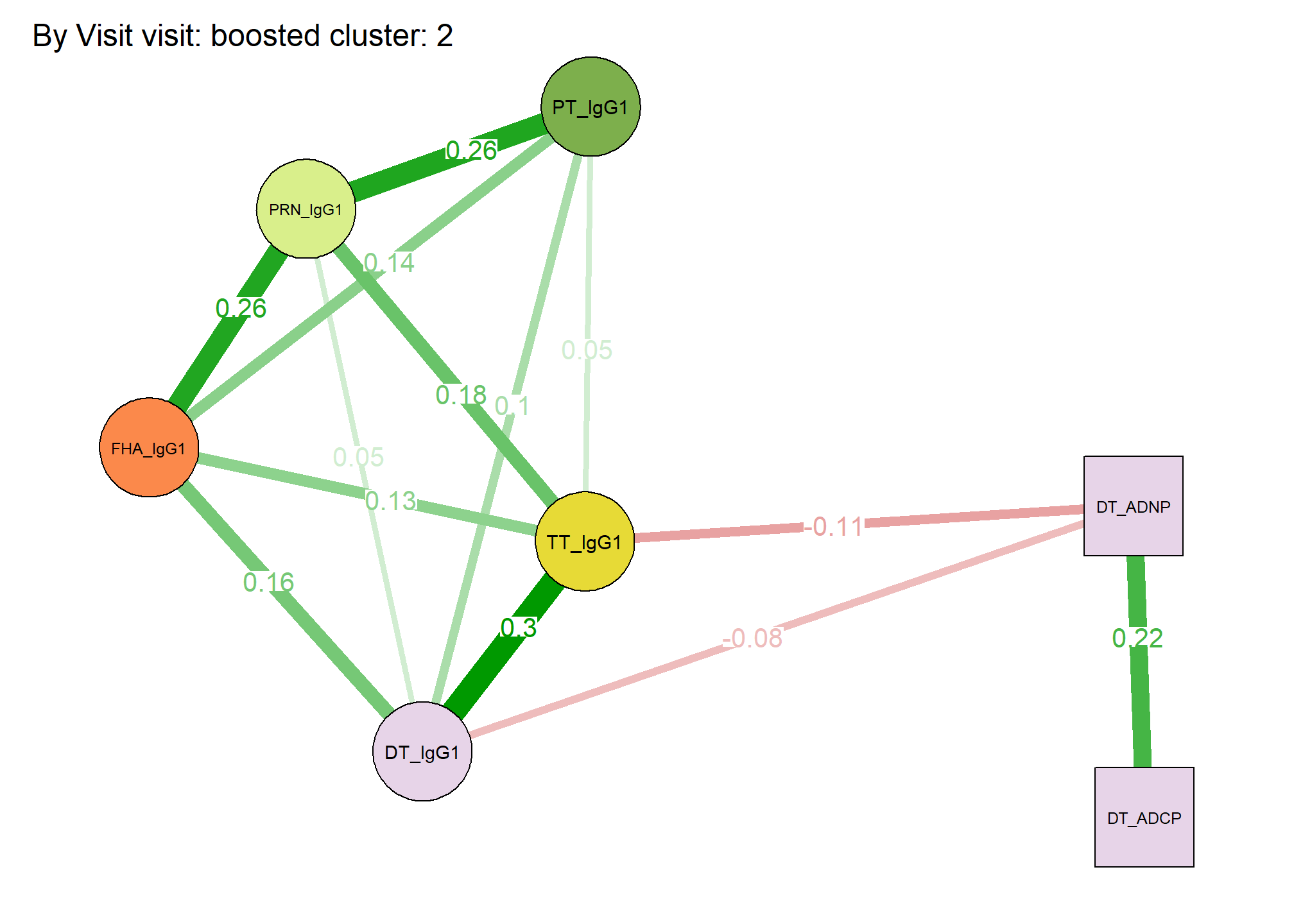 From
To Weight 1 — 2 0.22 2 — 3 -0.08 3 — 4 0.16 3 — 5 0.05 4 — 5 0.26 3 — 6
0.1 4 — 6 0.14 5 — 6 0.26 2 — 7 -0.11 3 — 7 0.3 4 — 7 0.13 5 — 7 0.18 6
— 7 0.05
From
To Weight 1 — 2 0.22 2 — 3 -0.08 3 — 4 0.16 3 — 5 0.05 4 — 5 0.26 3 — 6
0.1 4 — 6 0.14 5 — 6 0.26 2 — 7 -0.11 3 — 7 0.3 4 — 7 0.13 5 — 7 0.18 6
— 7 0.05
Heatmap Subjects Clustered 2
Heatmap Arm Assigned 2
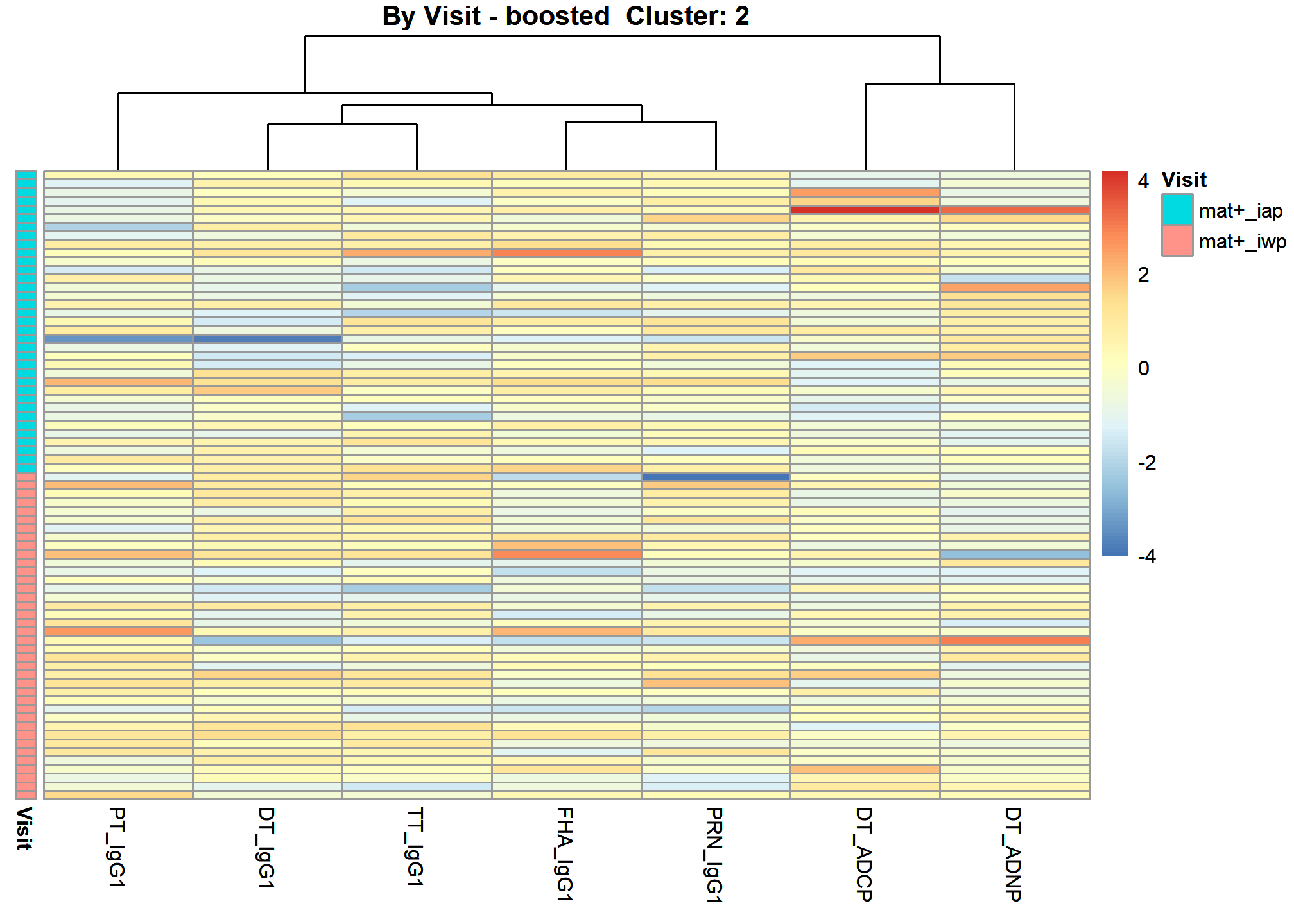
Cluster 3
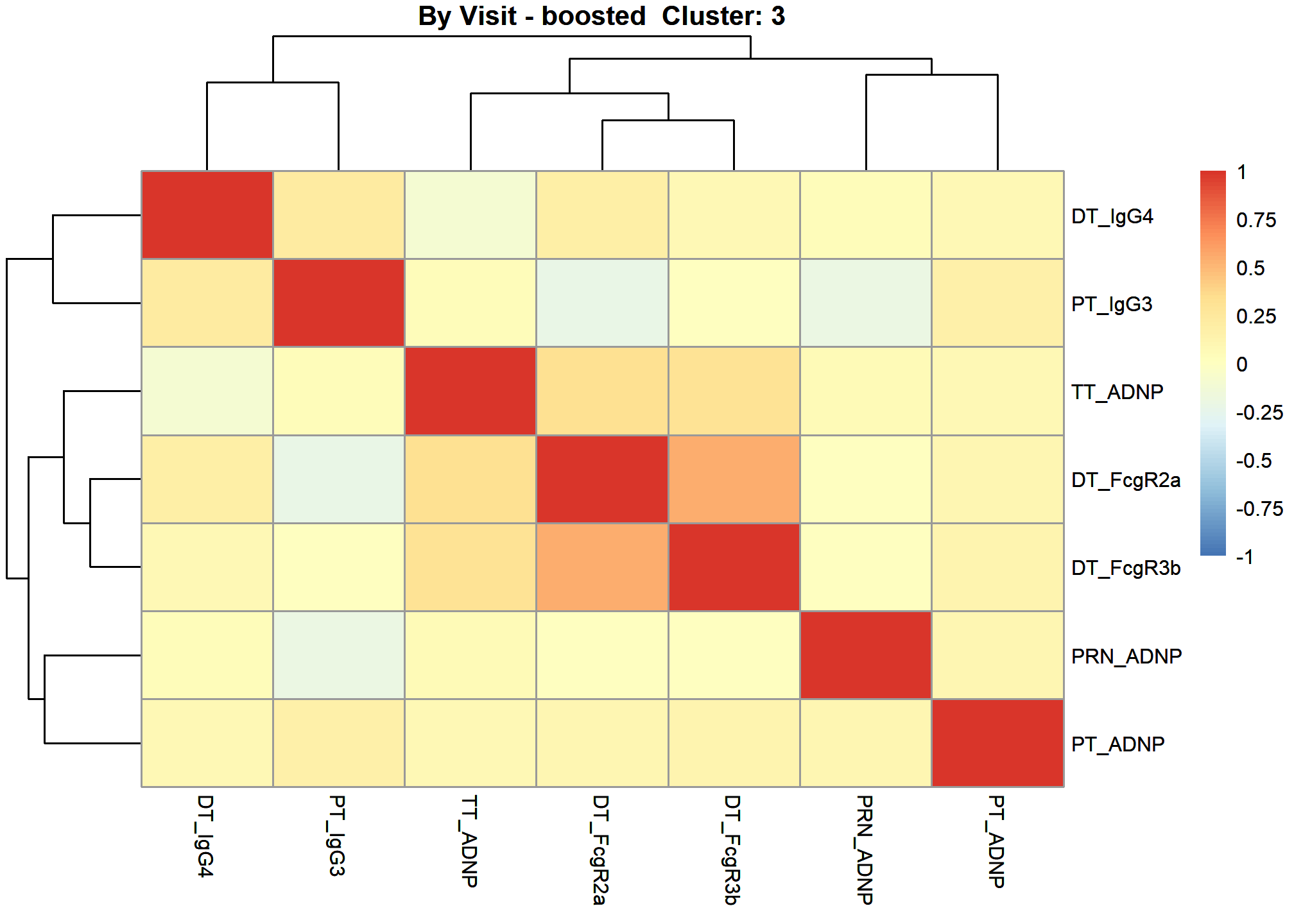
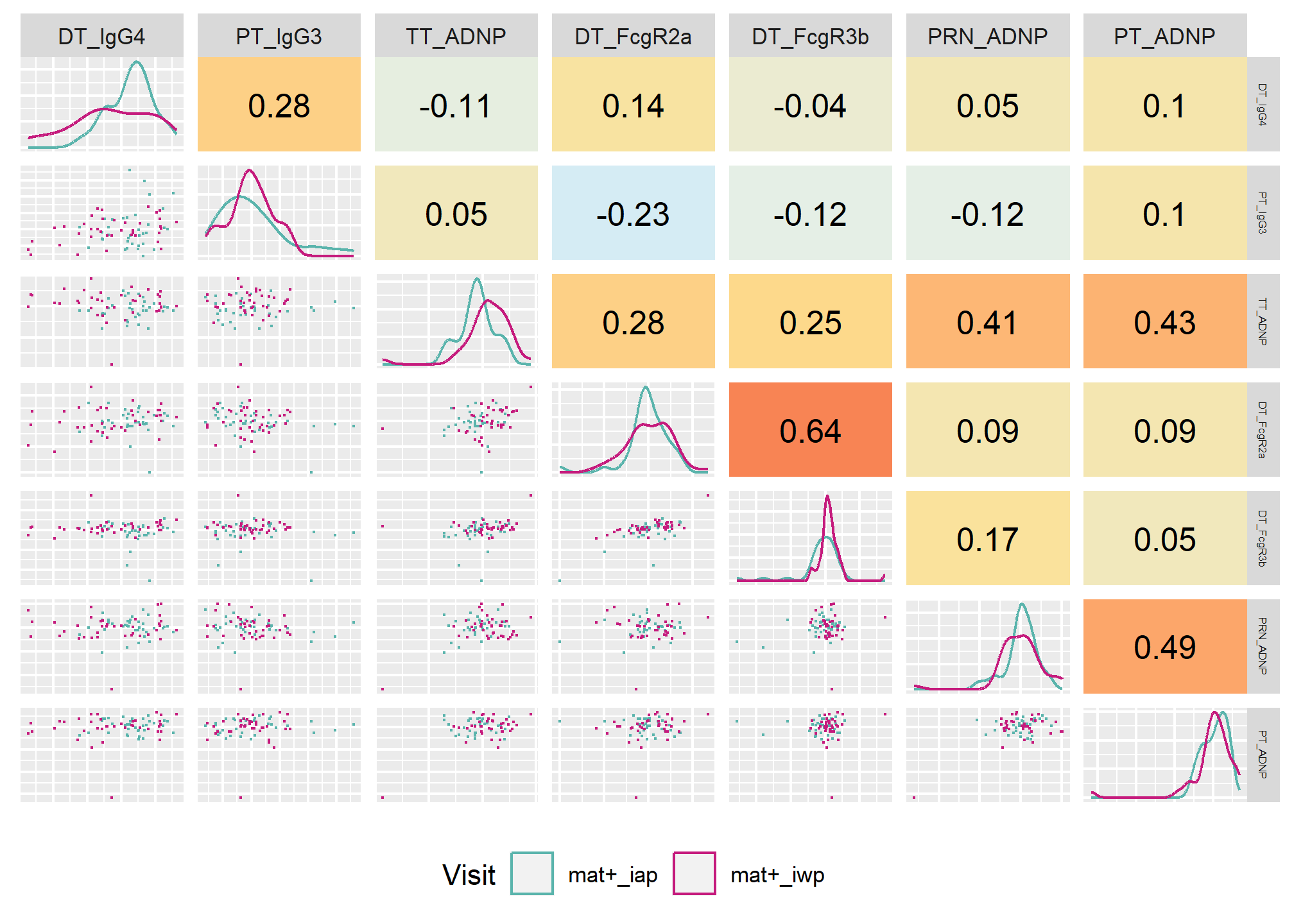
[1] “DT_FcgR2a” “DT_FcgR3b” “DT_IgG4” “PRN_ADNP” “PT_ADNP”
“PT_IgG3”
[7] “TT_ADNP”
Correlation Heatmap 3
These heatmaps are based on Spearman Rank Correlation.
 [1]
“after cluster specific correlation heatmap”
[1]
“after cluster specific correlation heatmap”
 [1]
“after cluster specific correlation scatter plot grid”
[1]
“after cluster specific correlation scatter plot grid”
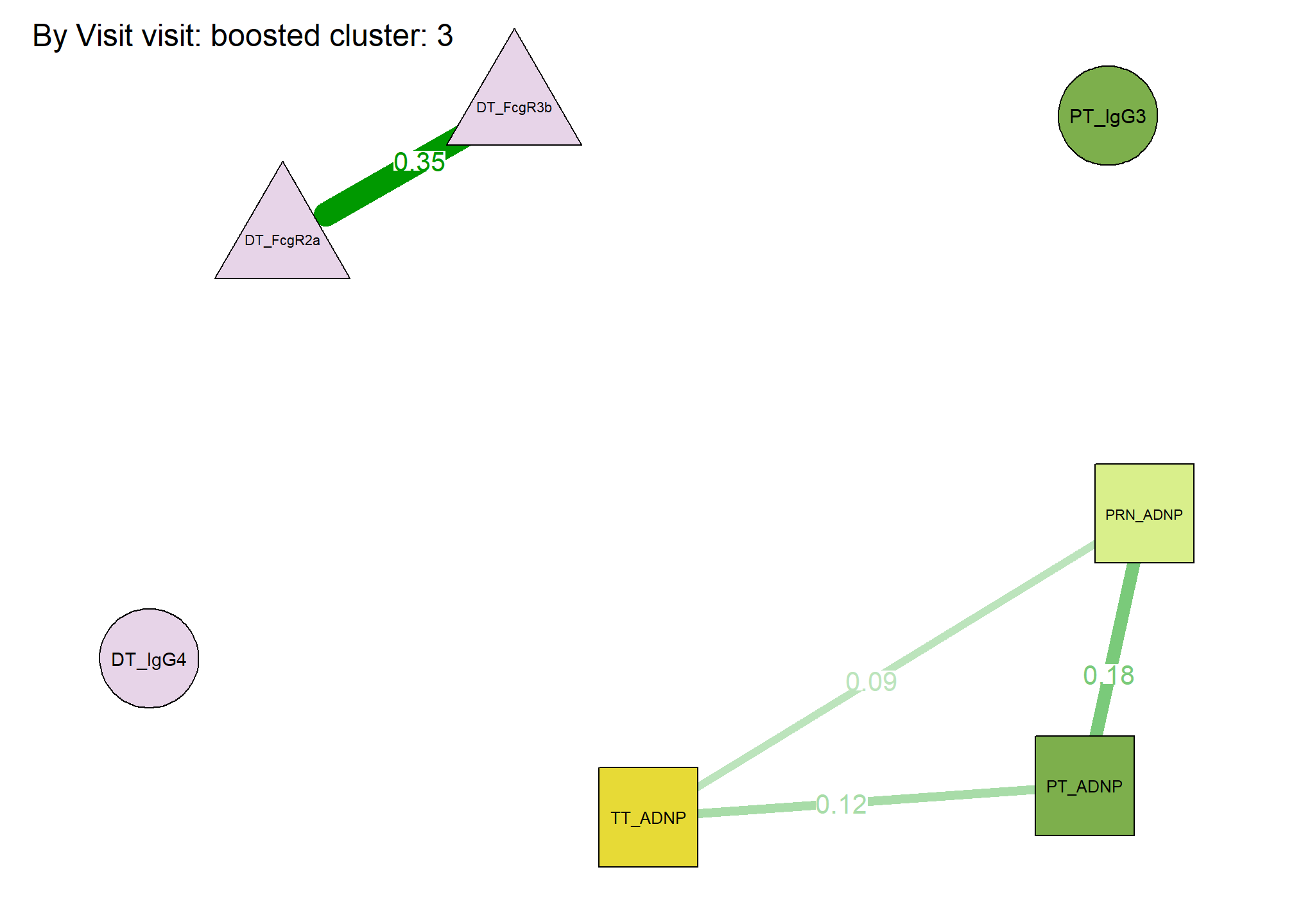
Correlation Network 3
The correlation networks are based on optimal sparse estimates of the partial correlation matrix (Friedman, Hastie and Tibshirani, 2011). Partial correlations represent the remaining association (-1,1) between two nodes after controlling for all other node associations (Epskamp, S. & Fried, Eiko I. (2018)). The lines between nodes are labelled with the partial correlation coefficient. Sometimes there are sparse networks when no significant partial correlation left to plot. Sometimes there are too few samples for the number of features and the correlation matrix becomes indefinite. In either of these circumstances no network plot will be made.
 From
To Weight 1 — 2 0.35 4 — 5 0.18 4 — 7 0.09 5 — 7 0.12
From
To Weight 1 — 2 0.35 4 — 5 0.18 4 — 7 0.09 5 — 7 0.12
Heatmap Subjects Clustered 3
Heatmap Arm Assigned 3
Cluster 4
[1] “DT_IgG2” “FHA_IgG2” “FHA_IgG4” “PRN_IgG2” “PRN_IgG4” “PT_IgG2” “PT_IgG4” [8] “TT_IgG2” “TT_IgG4”
Correlation Heatmap 4
These heatmaps are based on Spearman Rank Correlation.
 [1]
“after cluster specific correlation heatmap”
[1]
“after cluster specific correlation heatmap”
 [1]
“after cluster specific correlation scatter plot grid”
[1]
“after cluster specific correlation scatter plot grid”
Correlation Network 4
The correlation networks are based on optimal sparse estimates of the partial correlation matrix (Friedman, Hastie and Tibshirani, 2011). Partial correlations represent the remaining association (-1,1) between two nodes after controlling for all other node associations (Epskamp, S. & Fried, Eiko I. (2018)). The lines between nodes are labelled with the partial correlation coefficient. Sometimes there are sparse networks when no significant partial correlation left to plot. Sometimes there are too few samples for the number of features and the correlation matrix becomes indefinite. In either of these circumstances no network plot will be made.
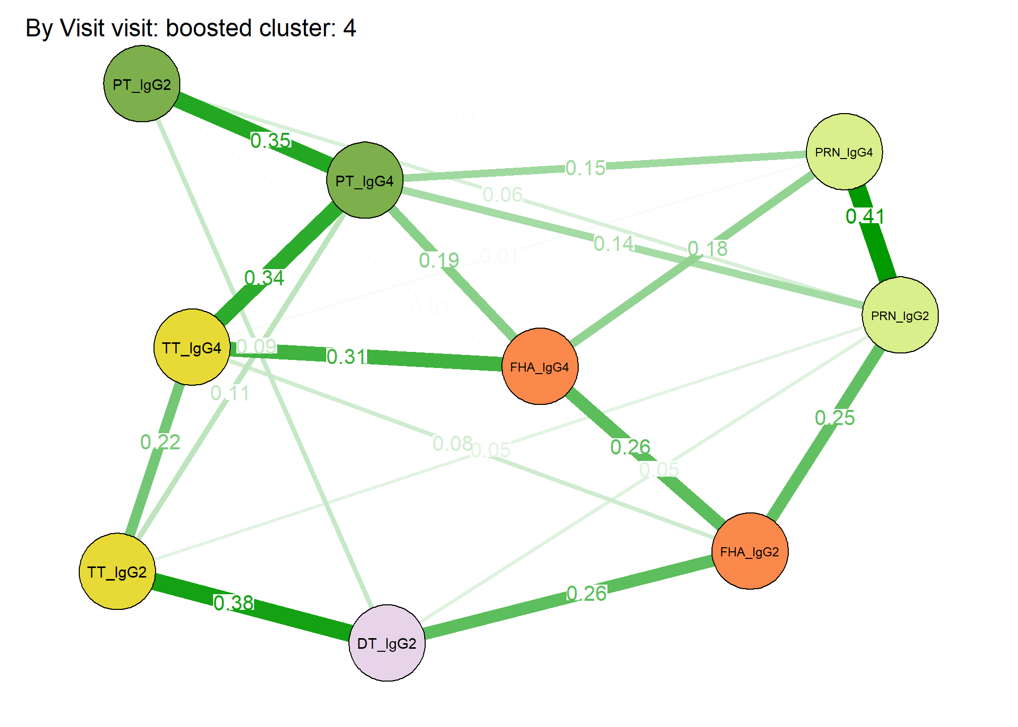 From
To Weight 1 — 2 0.26 2 — 3 0.26 1 — 4 0.05 2 — 4 0.25 3 — 5 0.18 4 — 5
0.41 1 — 6 0.09 2 — 6 0.01 4 — 6 0.06 5 — 6 0.01 3 — 7 0.19 4 — 7 0.14 5
— 7 0.15 6 — 7 0.35 1 — 8 0.38 2 — 8 0 4 — 8 0.05 7 — 8 0.11 2 — 9 0.08
3 — 9 0.31 5 — 9 0.01 7 — 9 0.34 8 — 9 0.22
From
To Weight 1 — 2 0.26 2 — 3 0.26 1 — 4 0.05 2 — 4 0.25 3 — 5 0.18 4 — 5
0.41 1 — 6 0.09 2 — 6 0.01 4 — 6 0.06 5 — 6 0.01 3 — 7 0.19 4 — 7 0.14 5
— 7 0.15 6 — 7 0.35 1 — 8 0.38 2 — 8 0 4 — 8 0.05 7 — 8 0.11 2 — 9 0.08
3 — 9 0.31 5 — 9 0.01 7 — 9 0.34 8 — 9 0.22
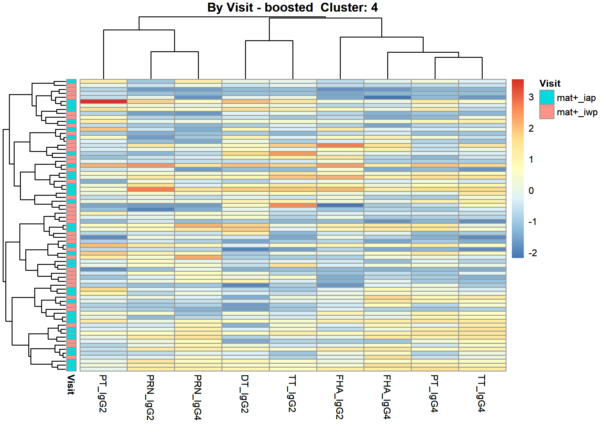
Heatmap Subjects Clustered 4
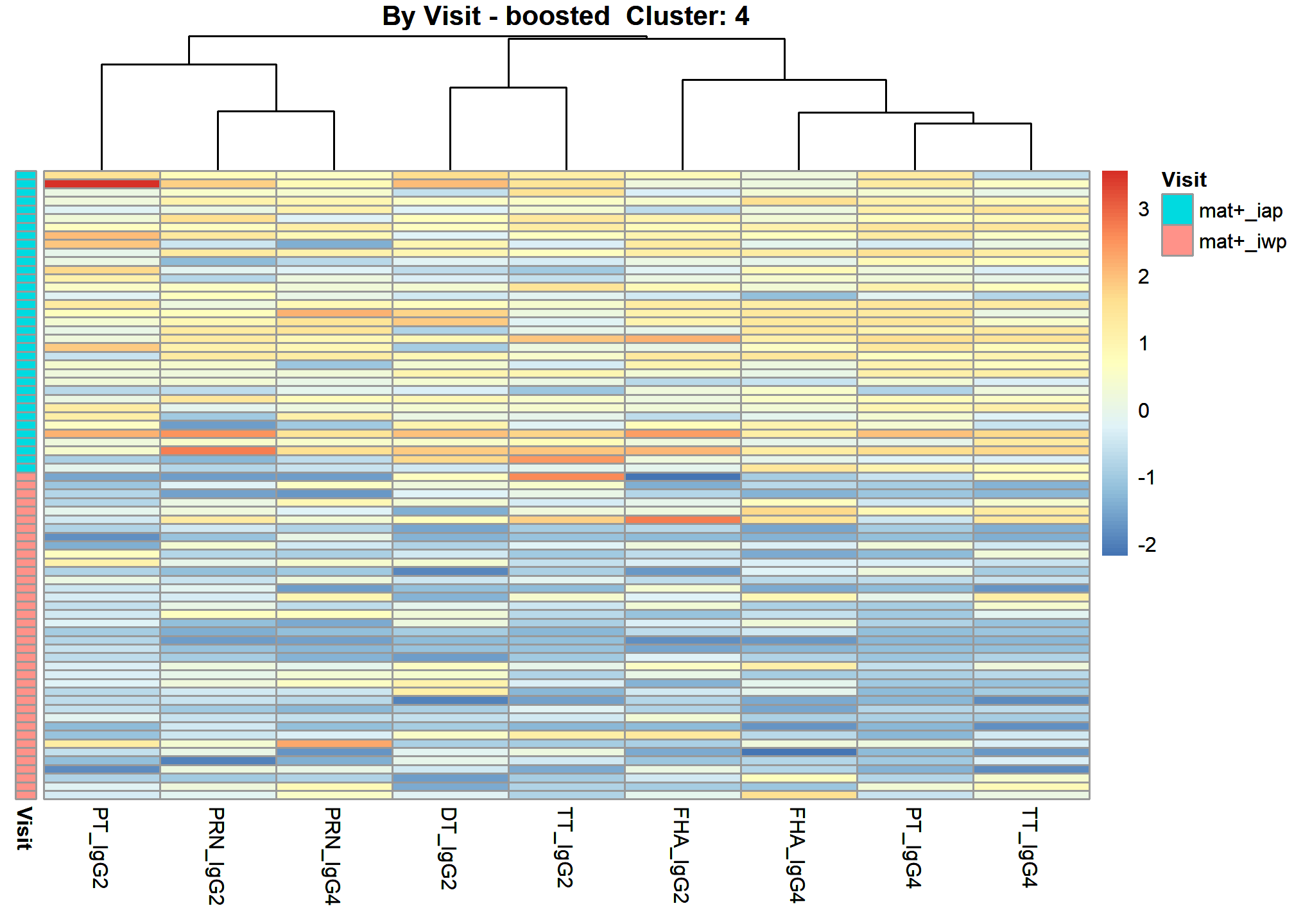
Heatmap Arm Assigned 4
Cluster 5
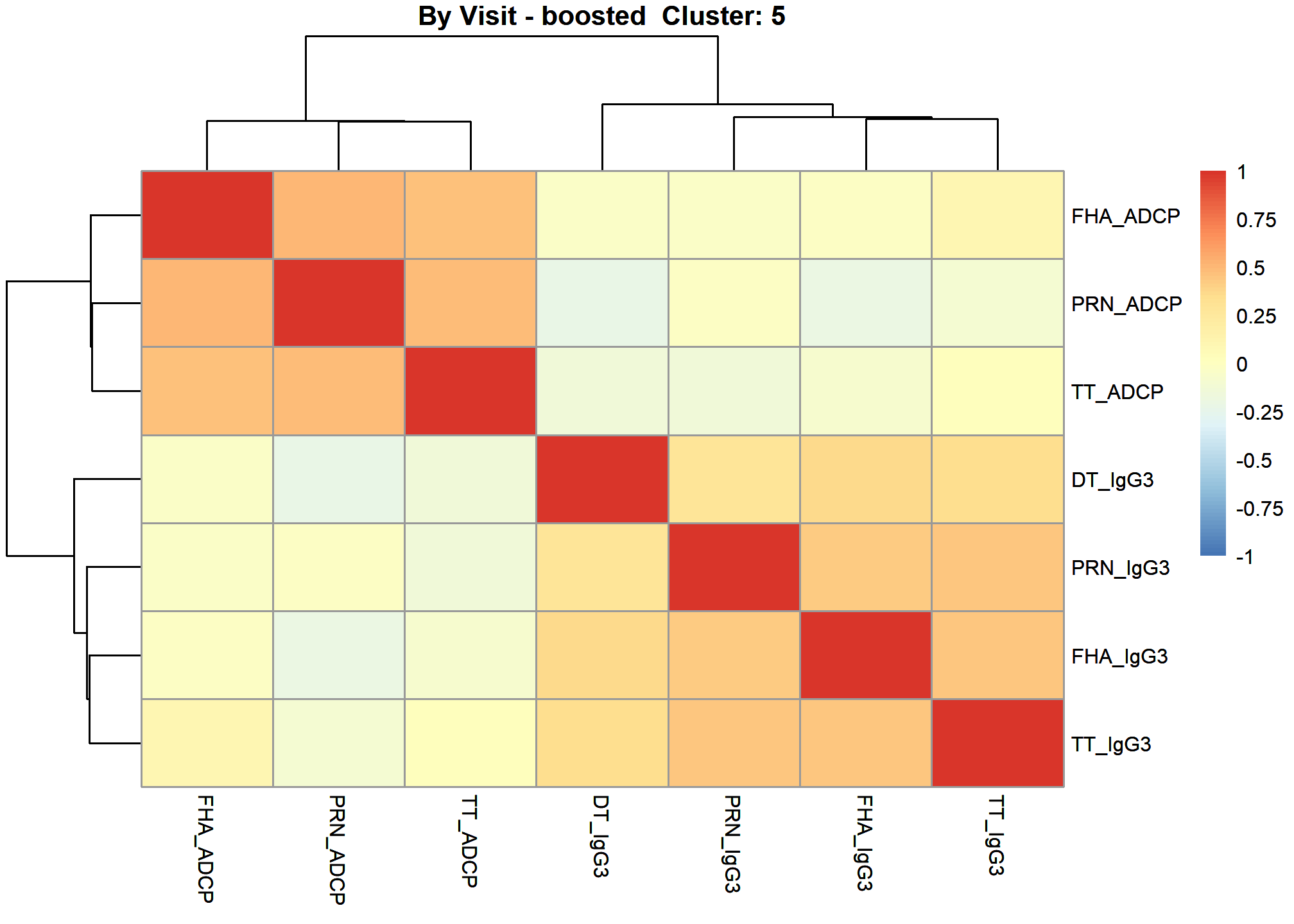
[1] “DT_IgG3” “FHA_ADCP” “FHA_IgG3” “PRN_ADCP” “PRN_IgG3” “TT_ADCP” “TT_IgG3”
Correlation Heatmap 5
These heatmaps are based on Spearman Rank Correlation.
 [1]
“after cluster specific correlation heatmap”
[1]
“after cluster specific correlation heatmap”
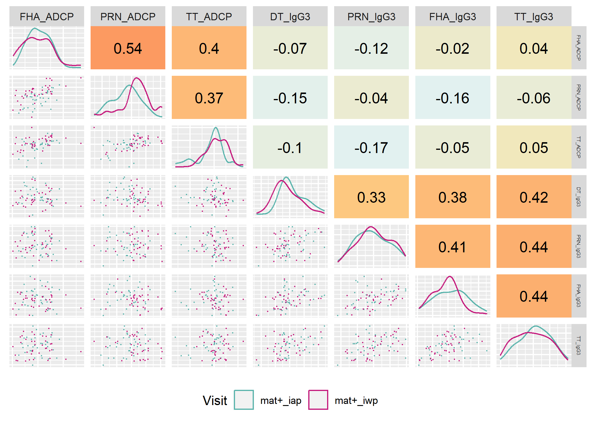 [1]
“after cluster specific correlation scatter plot grid”
[1]
“after cluster specific correlation scatter plot grid”
Correlation Network 5
The correlation networks are based on optimal sparse estimates of the partial correlation matrix (Friedman, Hastie and Tibshirani, 2011). Partial correlations represent the remaining association (-1,1) between two nodes after controlling for all other node associations (Epskamp, S. & Fried, Eiko I. (2018)). The lines between nodes are labelled with the partial correlation coefficient. Sometimes there are sparse networks when no significant partial correlation left to plot. Sometimes there are too few samples for the number of features and the correlation matrix becomes indefinite. In either of these circumstances no network plot will be made.
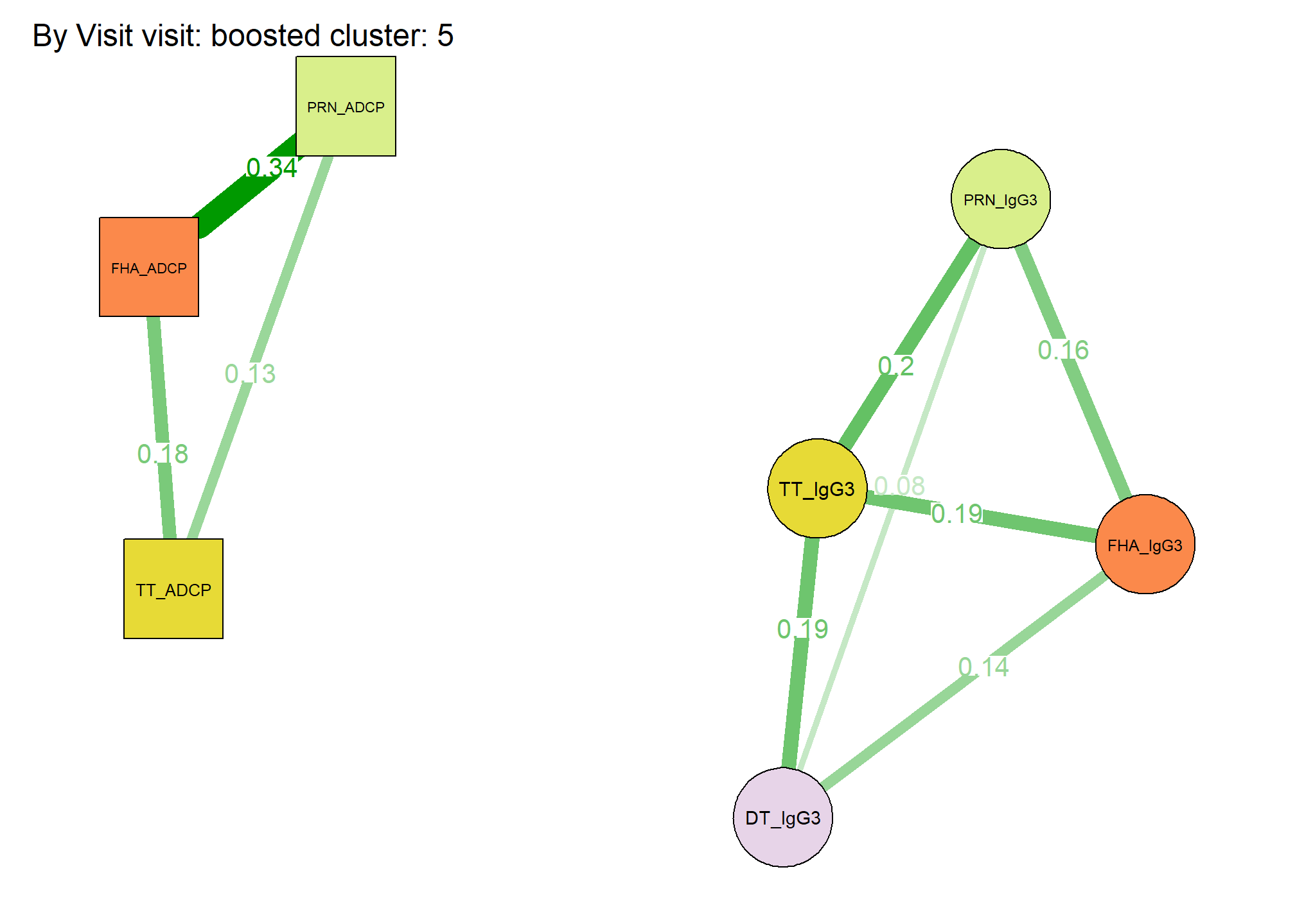 From
To Weight 1 — 3 0.14 2 — 4 0.34 1 — 5 0.08 3 — 5 0.16 2 — 6 0.18 4 — 6
0.13 1 — 7 0.19 3 — 7 0.19 5 — 7 0.2
From
To Weight 1 — 3 0.14 2 — 4 0.34 1 — 5 0.08 3 — 5 0.16 2 — 6 0.18 4 — 6
0.13 1 — 7 0.19 3 — 7 0.19 5 — 7 0.2
Heatmap Subjects Clustered 5
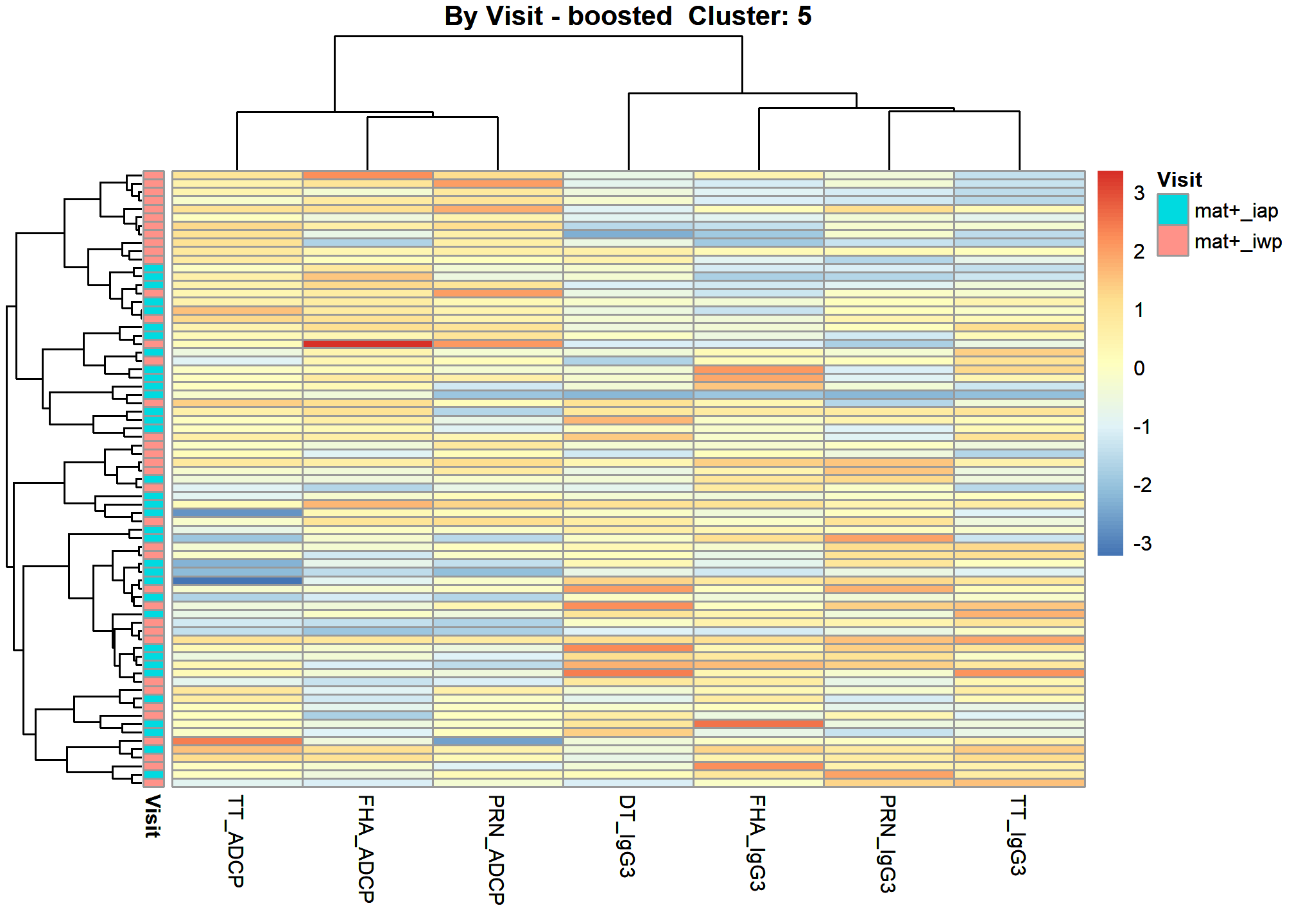
Heatmap Arm Assigned 5
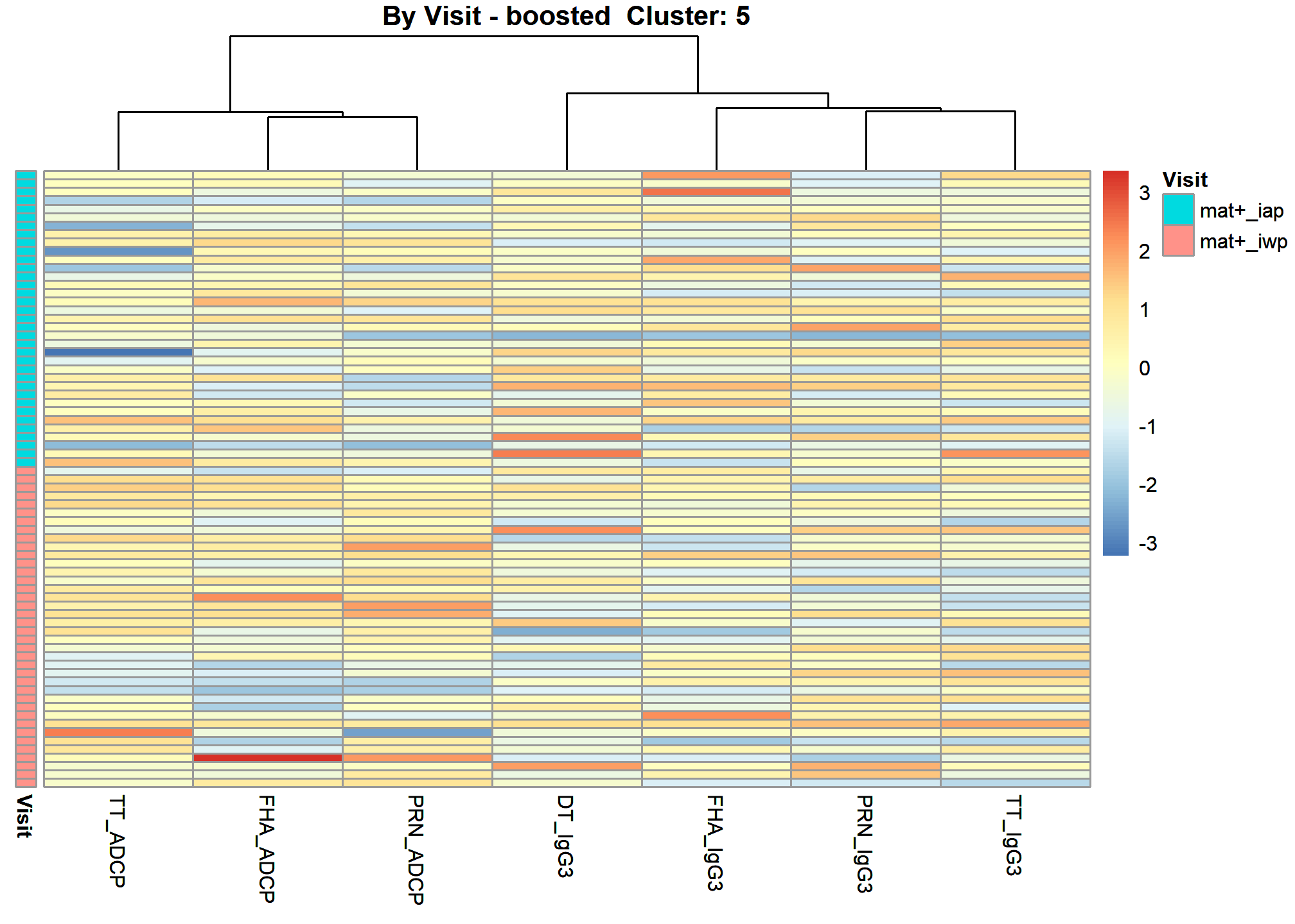
Cluster 6
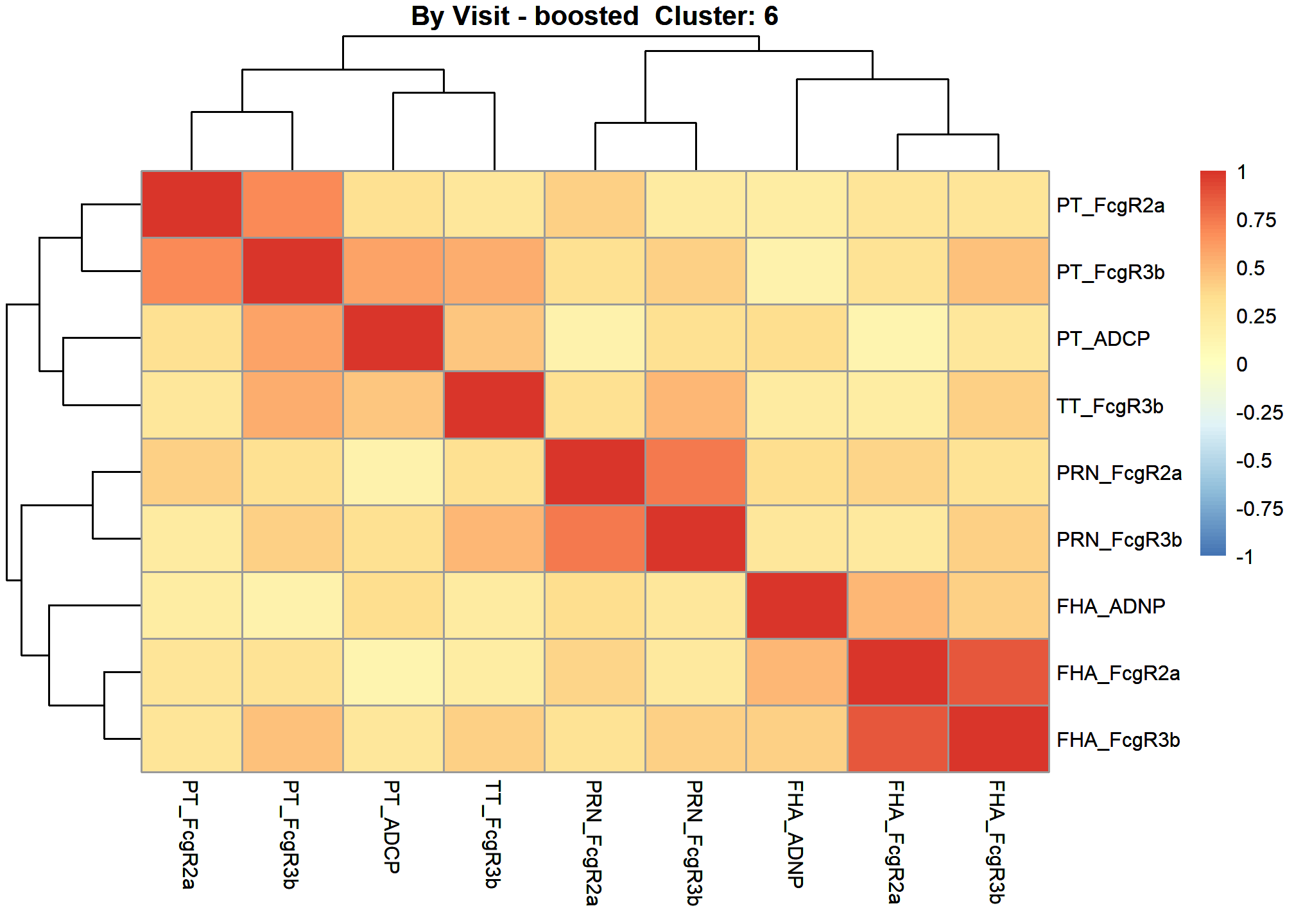
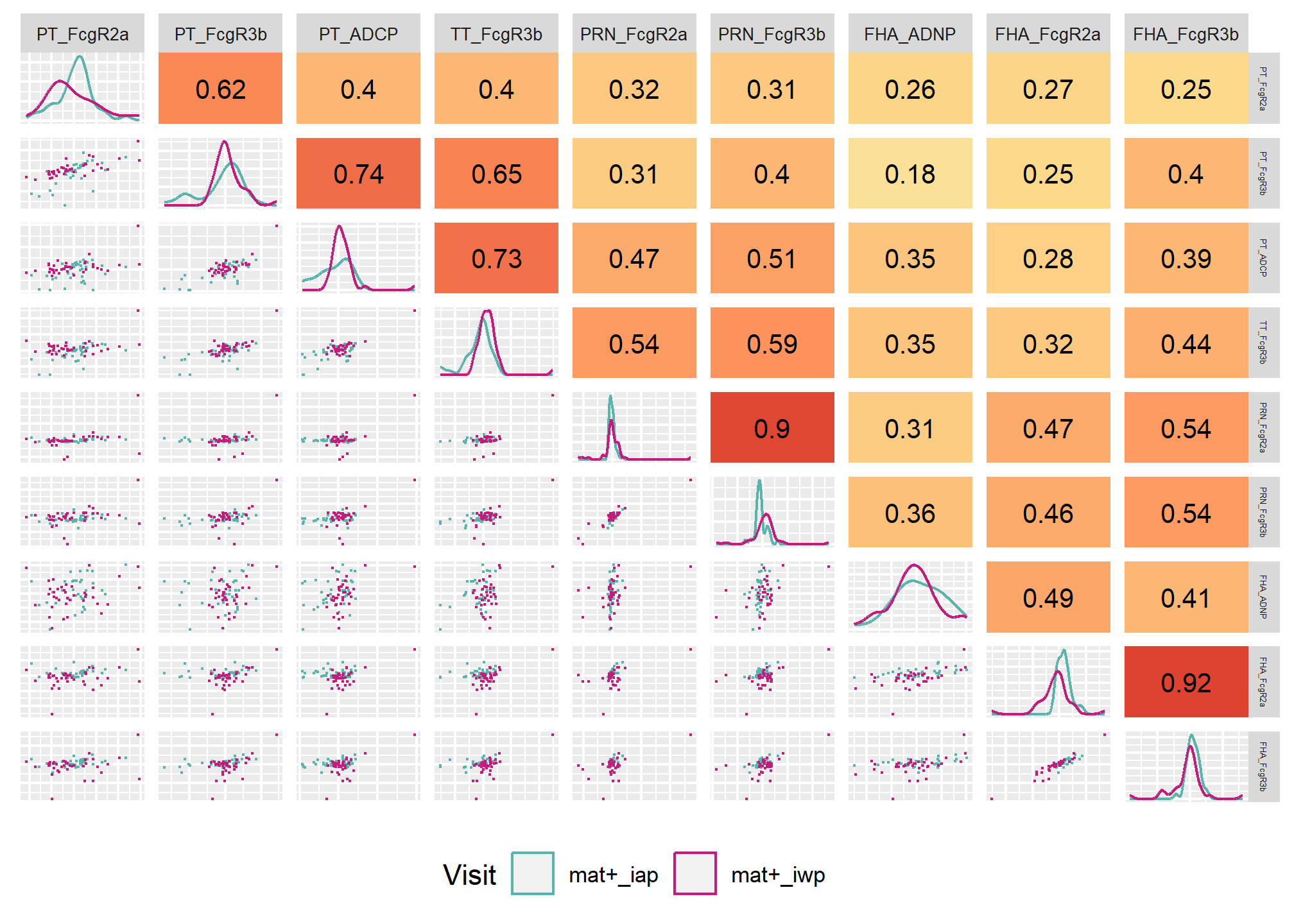
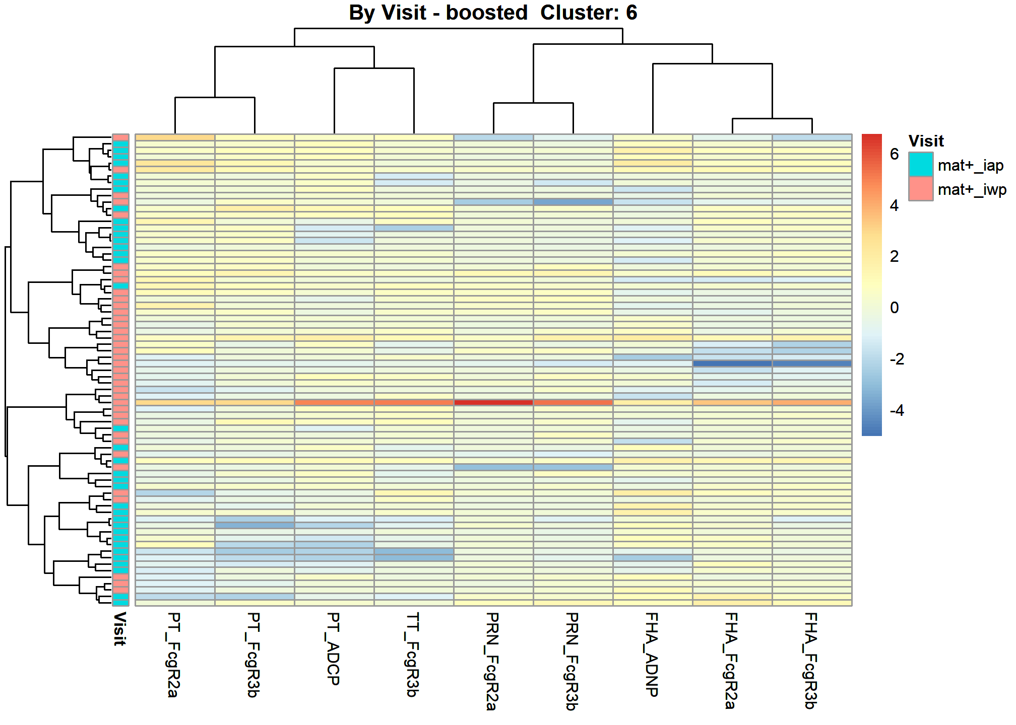
[1] “FHA_ADNP” “FHA_FcgR2a” “FHA_FcgR3b” “PRN_FcgR2a” “PRN_FcgR3b” [6] “PT_ADCP” “PT_FcgR2a” “PT_FcgR3b” “TT_FcgR3b”
Correlation Heatmap 6
These heatmaps are based on Spearman Rank Correlation.
 [1]
“after cluster specific correlation heatmap”
[1]
“after cluster specific correlation heatmap”
 [1]
“after cluster specific correlation scatter plot grid”
[1]
“after cluster specific correlation scatter plot grid”
Correlation Network 6
The correlation networks are based on optimal sparse estimates of the partial correlation matrix (Friedman, Hastie and Tibshirani, 2011). Partial correlations represent the remaining association (-1,1) between two nodes after controlling for all other node associations (Epskamp, S. & Fried, Eiko I. (2018)). The lines between nodes are labelled with the partial correlation coefficient. Sometimes there are sparse networks when no significant partial correlation left to plot. Sometimes there are too few samples for the number of features and the correlation matrix becomes indefinite. In either of these circumstances no network plot will be made.
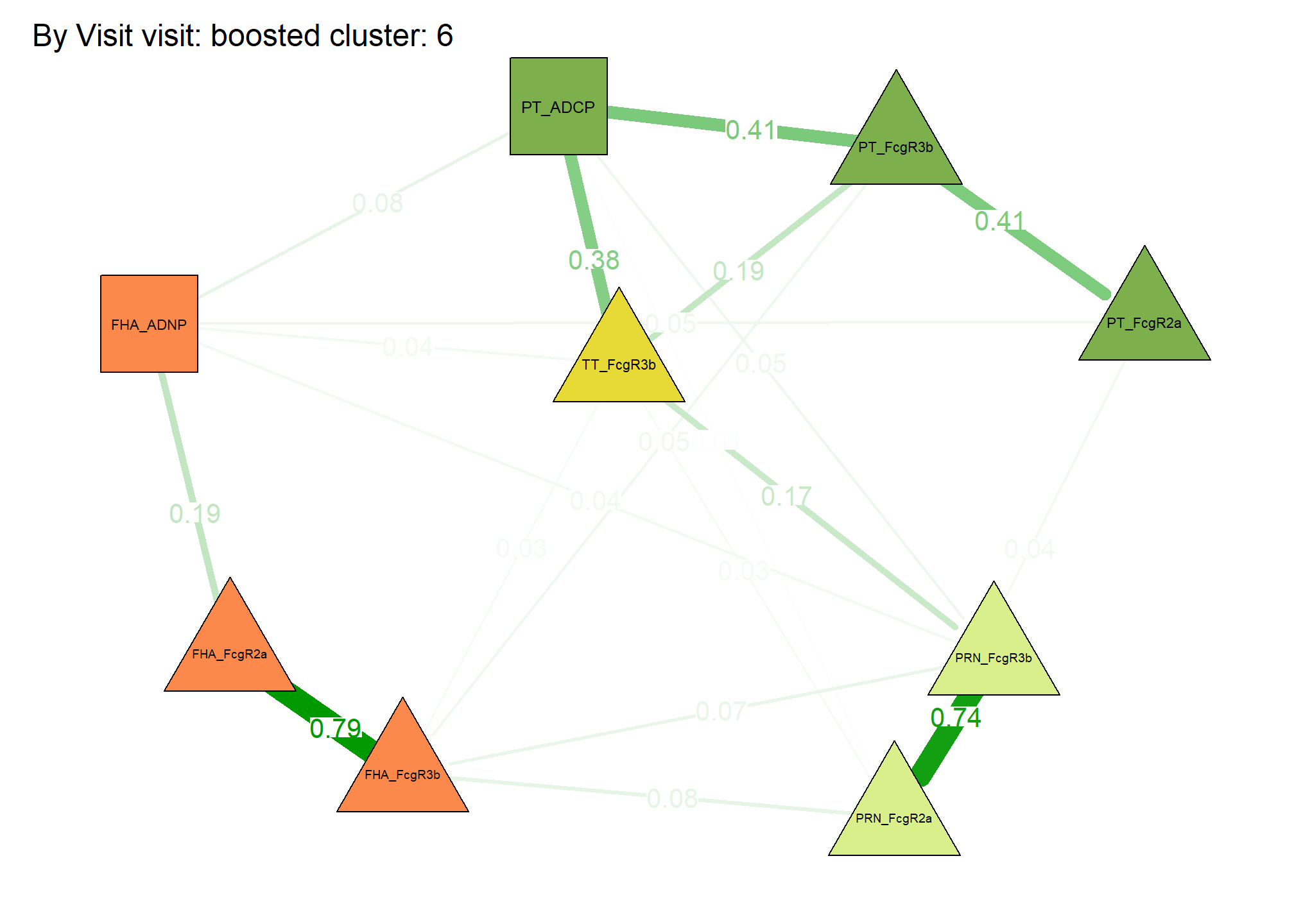 From
To Weight 1 — 2 0.19 2 — 3 0.79 3 — 4 0.08 1 — 5 0.04 3 — 5 0.07 4 — 5
0.74 1 — 6 0.08 4 — 6 0.01 5 — 6 0.05 1 — 7 0.05 2 — 7 0 4 — 7 0.04 3 —
8 0.05 6 — 8 0.41 7 — 8 0.41 1 — 9 0.04 3 — 9 0.03 4 — 9 0.03 5 — 9 0.17
6 — 9 0.38 8 — 9 0.19
From
To Weight 1 — 2 0.19 2 — 3 0.79 3 — 4 0.08 1 — 5 0.04 3 — 5 0.07 4 — 5
0.74 1 — 6 0.08 4 — 6 0.01 5 — 6 0.05 1 — 7 0.05 2 — 7 0 4 — 7 0.04 3 —
8 0.05 6 — 8 0.41 7 — 8 0.41 1 — 9 0.04 3 — 9 0.03 4 — 9 0.03 5 — 9 0.17
6 — 9 0.38 8 — 9 0.19
Heatmap Subjects Clustered 6
Heatmap Arm Assigned 6
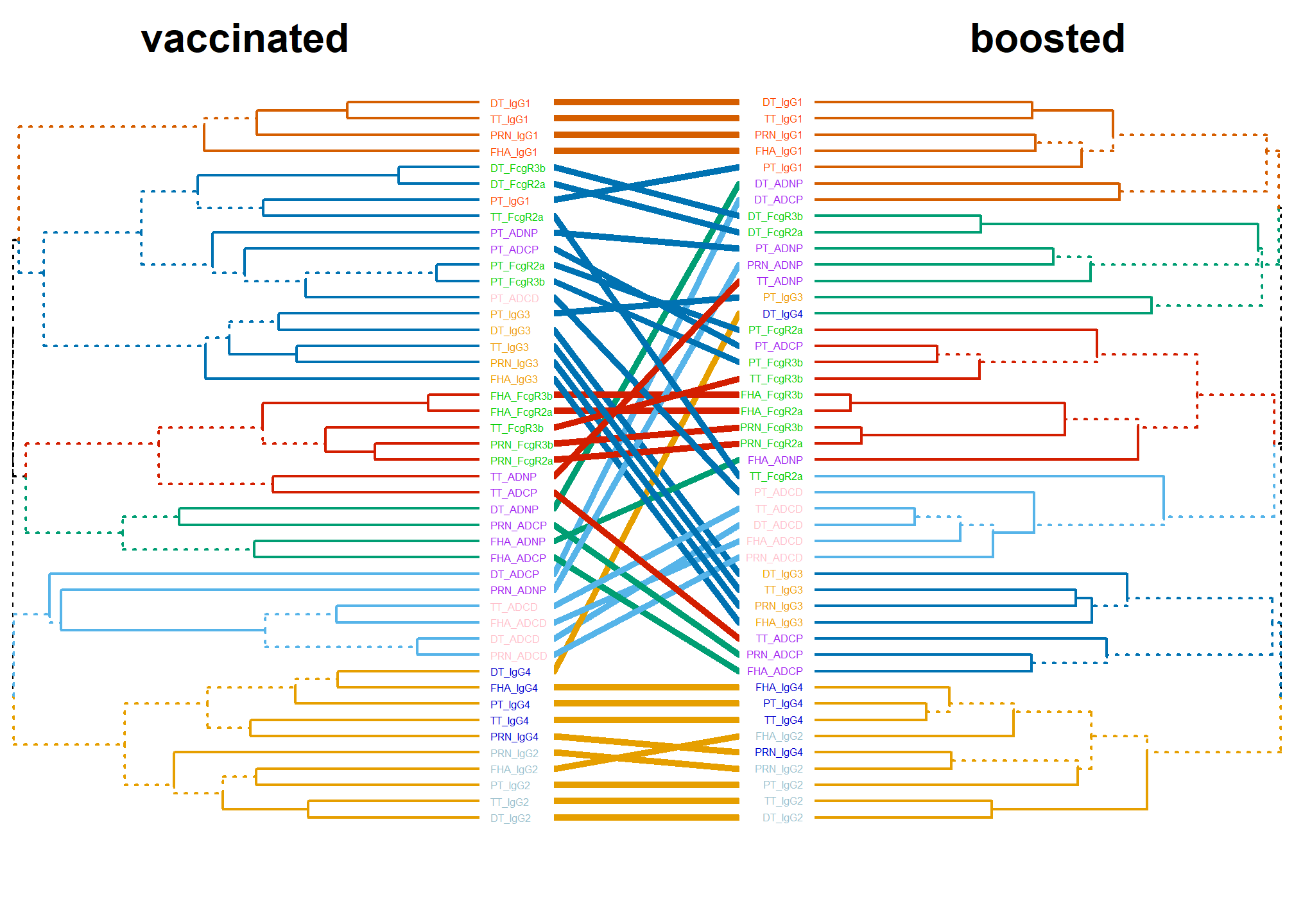
Compare dendrograms: By Visit
 $dend1
‘dendrogram’ with 2 branches and 45 members total, at height
0.9999476
$dend1
‘dendrogram’ with 2 branches and 45 members total, at height
0.9999476
$dend2 ‘dendrogram’ with 2 branches and 45 members total, at height 0.9998864
attr(,“class”) [1] “dendlist”
CRI: 0.227
MASTxCF: 0.07
RFS: 0.598
CRI (Clade Retention Index): The CRI quantifies agreement between two dendograms by counting the number of shared nodes and measures disagreement by counting the number of leaves that originate from an unshared node. The difference between these two counts is calculated and scaled relative to the maximum possible agreement.
MASTxCF (Maximum Agreement Subtree x Consensus Fork): MASTxCF begins by constructing the largest subtree that is fully agreed upon by two dendrograms, known as the Maximum Agreement Subtree (MAST). It then calculates the proportion of nodes from the original dendrogram that are included in this subtree. This value is multiplied by the proportion of nodes shared between the two trees, as measured by Colless’s Consensus Fork (CF).
RFS (Robinson-Foulds Similarity): RFS first calculates the Robinson-Foulds (RF) distance between two dendograms by counting the number of branch modifications (removals and additions) required to transform one tree into the other. This distance is scaled relative to the maximum possible RF distance for the given trees, then inverted so that a higher value indicates greater similarity between the dendrograms.All metrics quantify tree similarity on a scale from 0 to 1, where 1 corresponds to two trees being identical in structure.
Vidovic, S. U. (2019). Tree congruence: quantifying similarity between dendrogram topologies. ePrints|Soton. https://doi.org/10.5258/SOTON/D1069
sessionInfo()R version 4.3.1 (2023-06-16 ucrt)
Platform: x86_64-w64-mingw32/x64 (64-bit)
Running under: Windows 10 x64 (build 19045)
Matrix products: default
locale:
[1] LC_COLLATE=English_United States.utf8
[2] LC_CTYPE=English_United States.utf8
[3] LC_MONETARY=English_United States.utf8
[4] LC_NUMERIC=C
[5] LC_TIME=English_United States.utf8
time zone: America/New_York
tzcode source: internal
attached base packages:
[1] stats graphics grDevices utils datasets methods base
other attached packages:
[1] broom_1.0.5 e1071_1.7-13 glue_1.6.2 RPostgres_1.4.5
[5] RColorBrewer_1.1-3 phangorn_2.11.1 TreeDist_2.9.0 ape_5.8
[9] gt_0.10.1 ggforce_0.4.2 ggrepel_0.9.3 umap_0.2.10.0
[13] ggfortify_0.4.16 ppcor_1.1 MASS_7.3-60.0.1 phdcocktail_0.1.0
[17] gtsummary_1.7.2 ggpubr_0.6.0 rstatix_0.7.2 mvtnorm_1.2-3
[21] GGally_2.2.1 pvclust_2.2-0 rcompanion_2.4.34 polycor_0.8-1
[25] boot_1.3-28.1 qgraph_1.9.8 janitor_2.2.0 dendextend_1.17.1
[29] pheatmap_1.0.12 skimr_2.1.5 kableExtra_1.3.4 rmarkdown_2.25
[33] papeR_1.0-5 xtable_1.8-4 car_3.1-2 carData_3.0-5
[37] mclust_6.0.1 kohonen_3.0.12 clValid_0.7 cluster_2.1.6
[41] NbClust_3.0.1 data.table_1.14.8 DT_0.28 DBI_1.1.3
[45] fpc_2.2-10 extrafont_0.19 lubridate_1.9.2 forcats_1.0.0
[49] stringr_1.5.0 dplyr_1.1.2 purrr_1.0.1 readr_2.1.4
[53] tidyr_1.3.0 tibble_3.2.1 ggplot2_3.4.4 tidyverse_2.0.0
[57] here_1.0.1
loaded via a namespace (and not attached):
[1] bitops_1.0-7 fs_1.6.3 matrixStats_1.0.0
[4] httr_1.4.7 webshot_0.5.5 prabclus_2.3-3
[7] repr_1.1.6 tools_4.3.1 backports_1.4.1
[10] utf8_1.2.3 R6_2.5.1 nortest_1.0-4
[13] withr_3.0.0 gridExtra_2.3 fdrtool_1.2.17
[16] cli_3.6.1 shinyjs_2.1.0 sandwich_3.1-0
[19] labeling_0.4.3 sass_0.4.9 diptest_0.77-0
[22] robustbase_0.99-1 proxy_0.4-27 pbapply_1.7-2
[25] askpass_1.2.0 pbivnorm_0.6.0 systemfonts_1.0.5
[28] foreign_0.8-84 R.utils_2.12.2 svglite_2.1.2
[31] readxl_1.4.3 rstudioapi_0.15.0 generics_0.1.3
[34] gtools_3.9.4 Matrix_1.6-1.1 fansi_1.0.4
[37] DescTools_0.99.52 abind_1.4-5 R.methodsS3_1.8.2
[40] lifecycle_1.0.4 multcomp_1.4-25 yaml_2.3.7
[43] snakecase_0.11.1 blob_1.2.4 grid_4.3.1
[46] lavaan_0.6-16 PlotTools_0.3.1 promises_1.2.0.1
[49] gdata_2.19.0 lattice_0.21-8 pillar_1.9.0
[52] knitr_1.47 gld_2.6.6 corpcor_1.6.10
[55] admisc_0.33 codetools_0.2-19 fastmatch_1.1-4
[58] V8_4.4.1 broom.helpers_1.14.0 vctrs_0.6.3
[61] png_0.1-8 Rdpack_2.6.1 cellranger_1.1.0
[64] gtable_0.3.4 kernlab_0.9-32 cachem_1.0.8
[67] xfun_0.45 mime_0.12 rbibutils_2.2.16
[70] libcoin_1.0-10 survival_3.5-5 ellipsis_0.3.2
[73] TH.data_1.1-2 nlme_3.1-164 bit64_4.0.5
[76] gmodels_2.18.1.1 rprojroot_2.0.4 R.cache_0.16.0
[79] bslib_0.7.0 TreeTools_1.12.0 rpart_4.1.19
[82] colorspace_2.1-0 Hmisc_5.1-1 nnet_7.3-19
[85] Exact_3.2 mnormt_2.1.1 tidyselect_1.2.0
[88] curl_5.1.0 bit_4.0.5 compiler_4.3.1
[91] extrafontdb_1.0 git2r_0.32.0 rvest_1.0.3
[94] htmlTable_2.4.1 expm_0.999-7 xml2_1.3.5
[97] checkmate_2.2.0 scales_1.3.0 DEoptimR_1.1-3
[100] psych_2.3.9 lmtest_0.9-40 quadprog_1.5-8
[103] multcompView_0.1-9 digest_0.6.33 htmltools_0.5.8
[106] pkgconfig_2.0.3 jpeg_0.1-10 base64enc_0.1-3
[109] highr_0.11 fastmap_1.1.1 rlang_1.1.1
[112] htmlwidgets_1.6.2 shiny_1.7.4.1 farver_2.1.1
[115] jquerylib_0.1.4 zoo_1.8-12 jsonlite_1.8.7
[118] R.oo_1.25.0 RCurl_1.98-1.13 magrittr_2.0.3
[121] modeltools_0.2-23 Formula_1.2-5 munsell_0.5.0
[124] Rcpp_1.0.11 viridis_0.6.4 reticulate_1.37.0
[127] stringi_1.7.12 rootSolve_1.8.2.4 plyr_1.8.9
[130] flexmix_2.3-19 ggstats_0.5.1 parallel_4.3.1
[133] lmom_3.0 splines_4.3.1 hms_1.1.3
[136] igraph_1.5.1 ggsignif_0.6.4 reshape2_1.4.4
[139] stats4_4.3.1 evaluate_0.23 tzdb_0.4.0
[142] tweenr_2.0.3 httpuv_1.6.11 Rttf2pt1_1.3.12
[145] openssl_2.1.1 polyclip_1.10-6 coin_1.4-3
[148] RSpectra_0.16-1 later_1.3.1 glasso_1.11
[151] viridisLite_0.4.2 class_7.3-22 memoise_2.0.1
[154] workflowr_1.7.1 timechange_0.2.0 concaveman_1.1.0